For a mathematical explanation of the test, see e.g. here. However, such an explanation is not very useful for using the test in practice. Just what does a W value of .95 mean? What about .90 or .99? One way to get a feel for it, is to simulate datasets, plot them and calculate the W values. Additionally, one can check the sensitivity of the test, i.e. the p value.
All the code is in R.
#random numbers from normal distribution
set.seed(42) #for reproducible numbers
x = rnorm(5000) #generate random numbers from normal dist
hist(x,breaks=50, main="Normal distribution, N=5000") #plot
shapiro.test(x) #SW test
>W = 0.9997, p-value = 0.744
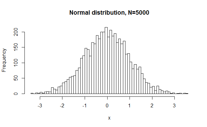
So, as expected, W was very close to 1, and p was large. In other words, SW did not reject a normal distribution just because N is large. But maybe it was a freak accident. What if we were to repeat this experiment 1000 times?
#repeat sampling + test 1000 times
Ws = numeric(); Ps = numeric() #empty vectors
for (n in 1:1000){ #number of simulations
  x = rnorm(5000) #generate random numbers from normal dist
  sw = shapiro.test(x)
  Ws = c(Ws,sw$statistic)
  Ps = c(Ps,sw$p.value)
}
hist(Ws,breaks=50) #plot W distribution
hist(Ps,breaks=50) #plot P distribution
sum(Ps<.05) #how many Ps below .05?
The number of Ps below .05 was in fact 43, or 4.3%. I ran the code with 100,000 simulations too, which takes 10 minutes or something. The value was 4389, i.e. 4.4%. So it seems that the method used to estimate the P value is slightly off in that the false positive rate is lower than expected.
What about the W statistic? Is it sensitive to fairly small deviations from normality?
#random numbers from normal distribution, slight deviation
x = c(rnorm(4900),rnorm(100,2))
hist(x,breaks=50, main="Normal distribution N=4900 + normal distribution N=200, mean=2")
shapiro.test(x)
>W = 0.9965, p-value = 1.484e-09
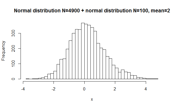
Here I started with a very large norm. dist. and added a small norm dist. to it with a different mean. The difference is hardly visible to the eye, but the P value is very small. The reason is that the large sample size makes it possible to detect even very small deviations from normality. W was again very close to 1, indicating that the distribution was close to normal.
What about a decidedly non-normal distribution?
#random numbers between -10 and 10
x = runif(5000, min=-10, max=10)
hist(x,breaks=50,main="evenly distributed numbers [-10;10], N=5000")
shapiro.test(x)
>W = 0.9541, p-value < 2.2e-16
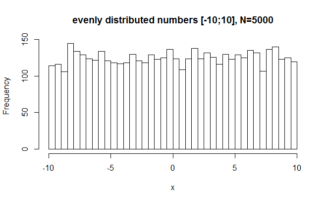
SW wisely rejects this with great certainty as being normal. However, W is near 1 still (.95). This tells us that the W value does not vary very much even when the distribution is decidedly non-normal. For interpretation then, we should probably bark when W drops just under .99 or so.
As a further test of the W values, here’s two equal sized distributions plotted together.
#normal distributions, 2 sd apart (unimodal fat normal distribution)
x = c(rnorm(2500, -1, 1),rnorm(2500, 1, 1))
hist(x,breaks=50,main="Mormal distributions, 2 sd apart")
shapiro.test(x)
>W = 0.9957, p-value = 6.816e-11
sd(x)
>1.436026
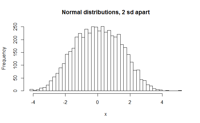 It still looks fairly normal, altho too fat. The standard deviation is in fact 1.44, or 44% larger than it is supposed to be. The W value is still fairly close to 1, however, and only a little less than from the distribution that was only slightly nonnormal (Ws = .9957 and .9965). What about clearly bimodal distributions?
#bimodal normal distributions, 4 sd apart
x = c(rnorm(2500, -2, 1),rnorm(2500, 2, 1))
hist(x,breaks=50,main="Normal distributions, 4 sd apart")
shapiro.test(x)
>W = 0.9464, p-value < 2.2e-16
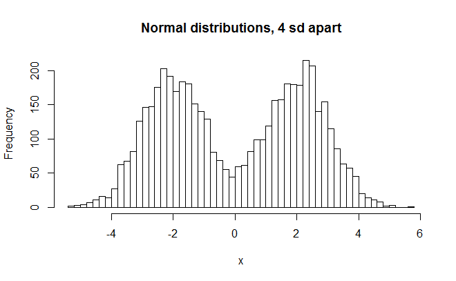
This clearly looks nonnormal. SW rejects it rightly and W is about .95 (W=0.9464). This is a bit lower than for the evenly distributed numbers. (W=0.9541)
What about an extreme case of nonnormality?
#bimodal normal distributions, 20 sd apart
x = c(rnorm(2500, -10, 1),rnorm(2500, 10, 1))
hist(x,breaks=50,main="Normal distributions, 20 sd apart")
shapiro.test(x)
>W = 0.7248, p-value < 2.2e-16
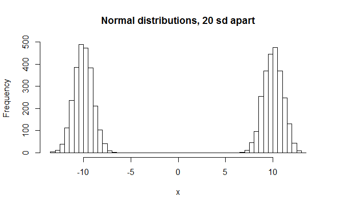
Finally we make a big reduction in the W value.
What about some more moderate deviations from normality?
#random numbers from normal distribution, moderate deviation
x = c(rnorm(4500),rnorm(500,2))
hist(x,breaks=50, main="Normal distribution N=4500 + normal distribution N=500, mean=2")
shapiro.test(x)
>W = 0.9934, p-value = 1.646e-14
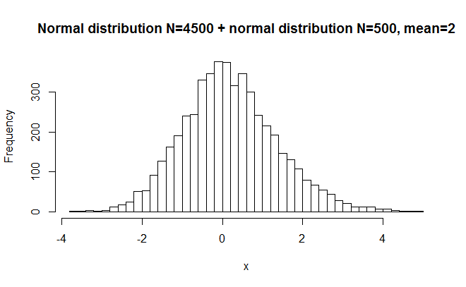
This one has a longer tail on the right side, but it still looks fairly normal. W=.9934.
#random numbers from normal distribution, large deviation
x = c(rnorm(4000),rnorm(1000,2))
hist(x,breaks=50, main="Normal distribution N=4000 + normal distribution N=1000, mean=2")
shapiro.test(x)
>W = 0.991, p-value < 2.2e-16
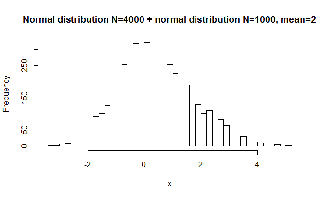
This one has a very long right tail. W=.991.
In conclusion
Generally we see that given a large sample, SW is sensitive to departures from non-normality. If the departure is very small, however, it is not very important.
We also see that it is hard to reduce the W value even if one deliberately tries. One needs to test extremely non-normal distribution in order for it to fall appreciatively below .99.
