I looked around to see if I could find a nice function for just plotting the results of kmeans() using ggplot2. I could not find that. So I wrote my own function.
The example data I’m using is real GDP growth, not sure exactly what it is, but the file can be found here: OECD real economic growth. The datafile: GDP. Because some data is missing, I use imputation using irmi() from VIM.
One thing about kmeans is that it is an indeterministic algorithm because it depends on an initial position of the cluster means. In the default settings, these are picked at random. This means that results won’t be completely identical always. Even when they are, factors may be change numbers. Such is life. We can get around that by running the method a large number of times and picking the best of the solutions found. I set the default for this to 100 runs.
kmeans can use raw data if desired. Generally however this is not desired. That is, we want all the data to count equally, not differ in importance because their scales are different. The default setting is thus to standardize the data first.
Then there is the question of how to plot the solution. The usual solution is a scatter plot. I used that as well. The scatter plot is based on the two first factors as found by fa() (psych package).
Finally, I color code the factors and add rownames to the points for easy identification.
The results:


In the first plot, I have clustered the countries. In the second I have clustered the years. This is simply done by first transposing the dataset.
R code
library(pacman)
p_load(kirkegaard, psych, plyr, stringr, weights, VIM, ggplot2, readODS)

#read from file
d = read.ods("GDP.ods", 1)

#fix names
row_names = d$A[-1]
col_names = d[1, -1]
d = d[-1, -1]

#recode NA
d[d==""] = NA

#to numeric
d = as.data.frame(lapply(d, as.numeric))

#impute NA
d = irmi(d, noise = F)

#names
rownames(d) = row_names
colnames(d) = col_names

#transposed version
d2 = as.data.frame(t(d))

#some cors
round(wtd.cors(d), 2)
round(wtd.cors(t(d)), 2)

plot_kmeans = function(df, clusters, runs, standardize=T) {
  library(psych)
  library(ggplot2)

  #standardize
  if (standardize) df = std_df(df)

  #cluster
  tmp_k = kmeans(df, centers = clusters, nstart = 100)

  #factor
  tmp_f = fa(df, 2, rotate = "none")

  #collect data
  tmp_d = data.frame(matrix(ncol=0, nrow=nrow(df)))
  tmp_d$cluster = as.factor(tmp_k$cluster)
  tmp_d$fact_1 = as.numeric(tmp_f$scores[, 1])
  tmp_d$fact_2 = as.numeric(tmp_f$scores[, 2])
  tmp_d$label = rownames(df)

  #plot
  g = ggplot(tmp_d, aes(fact_1, fact_2, color = cluster)) + geom_point() + geom_text(aes(label = label), size = 3, vjust = 1, color = "black")
  return(g)
}

plot_kmeans(d, 2)
ggsave("cluster_GDP1.png")
plot_kmeans(d2, 2)
ggsave("cluster_GDP2.png")