I read the following interesting paper:
- Braun, S. T., & Stuhler, J. (2016). The Transmission of Inequality Across Multiple Generations: Testing Recent Theories with Evidence from Germany. The Economic Journal, n/a-n/a. https://doi.org/10.1111/ecoj.12453
This paper shows that across multiple generations, the persistence of occupational and educational attainment in Germany is larger than estimates from two generations suggest. We consider two recent interpretations. First, we assess Gregory Clark’s hypotheses that the true rate of intergenerational persistence is higher than the observed rate, as high as 0.75, and time-invariant. Our evidence supports the first but not the other two hypotheses. Second, we test for independent effects of grandparents. We show that the coefficient on grandparent status is positive in a wide class of Markovian models, and present evidence against its causal interpretation.
For some reason, they don’t report their numeric results in the abstract, but they find that the ‘persistence’ is about .60. They call it the heritability, but that’s an error because they can’t actually differentiate between genetics and environmental causation. I take it that the authors are not familiar with behavioral genetics. It’s weird that economists who try to work this stuff out don’t read the behavioral genetics literature, but instead try to reinvent methods. But I digress.
The good thing about this paper is that they come close to modeling the situation as I would i.e. with latent variables. They write:
Two distinct theories have gained particular attention. Clark (2014) and Clark and Cummins (2014) argue that wealth, education or occupational status is transmitted via an underlying and unobserved latent factor. They suggest that the persistence of this underlying factor is not only very high–much higher than the persistence in observed outcomes between parents and children–but also steady across social systems and time. Mare (2011) points to a very different interpretation of multigenerational correlations. He argues that the previous literature suffers from a fundamental conceptual limitation in that it considers only the transmission between parents and children. Following his call to overcome this “two-generation paradigm”, a fast-growing literature examines the existence of independent causal effects from other family members, in particular grandparents.
As usual, economists are fond of presenting their ideas in hard to understand jargon. They present the model as:
To capture this idea in a simple way, suppose that the intergenerational transmission of observable outcome yi,t and unobservable endowment ei,t in a one-parent one-offspring family is governed by
yi,t = ρei,t + ui,t (2)
ei,t = λei,t-1 + vi,t (3)
where ui,t and vi,t are noise terms that are uncorrelated with other variables and past values. For simplicity, we normalise the variances of yi,t and ei,t to one, so that slope coefficients can be interpreted as correlations. In this “latent factor model”, the offspring inherits her unobserved endowment from the parent (according to the “heritability” coefficient λ), and the endowment then translates into the observed outcome (according to the “transferability” coefficient ρ). The observed correlation in outcome y between generation t and generation t – m equals then
b-m = Cov(yi,t,yi,t-m)
= ρ2Cov(ei,t,ei,t-m)
= ρ2λm (4)
The persistence of socio-economic status over generations thus decreases with both the persistence of the unobserved endowment, as captured by
λ = Cov(ei,t, ei,t-m),
and the transferability of the unobserved endowment into the observed outcome, as captured by ρ. Across multiple generations, however, persistence is predominantly governed by λ rather than ρ. This is because the latent factor ei,t is inherited m times across generations but only twice transformed into outcome yi,t.
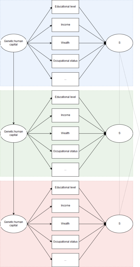
Hard to make sense of? Actually, it’s simpler to understand if one draws a SEM and changes it to use 2 latent variables instead of 1:
Each colored box is one generation, so the figure has 3 generations: blue, green and red. Each box is some aspect of socioeconomic inequality whether it be education, income or whatever. They are the indicators in factor analytic terms. The 2 circles are the latent variables. The first is genetic human capital, GHC, which is some mix of cognitive ability, work ethic, interests, preferences, personality but probably mostly the first. This is the part that parents actually transmit to their children. As people grow up and find their spot in society, they attain some socioeconomic outcomes which are correlated, and if we factor analyze them, we get the S factor I’ve been talking so much about. S is a formative factor, meaning that it doesn’t cause stuff; it’s basically an optimally weighted index of one’s relative social status. It has exactly the same indicators and loadings as the actual cause, GHC, and so the relative standing is exactly the same on these constructs if one can measure them without error.
Now we are able to easily explain traditional studies of intergenerational stability. They pick a single box, an indicator of S, and then correlate it between parents and children (average of parents and children if possible). This underestimates the actual stability because these single measures of S do not have factor loadings of 1.00. The actual realized stability is given by causal paths between each generation’s S scores. Grandparents only transmit genes to their grandchildren thru their own children, so there is no causal path from generation blue GHC to generation red GHC, but one can of course correlate them, shown by the dotted line between generation blue’s S and generation red’s S.
In their terms, they call the arrows between GHC for the heritability (that’s also technically correct in my model) and they call the factor loadings for the transferability.
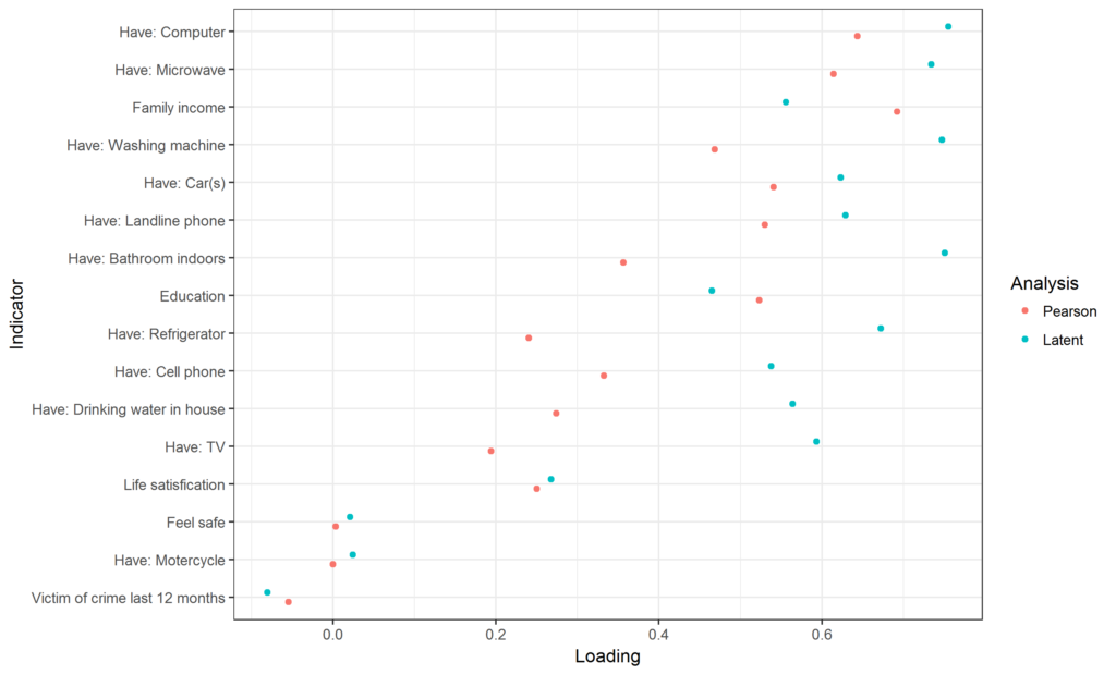
To estimate the GHC path(s), one then has to gather a diverse set of socioeconomic indicators for each person, factor analyze them, and correlate the S scores across generations. Usually, it is hard to get this kind of data, so researchers only rely on single variables instead. One can do this, but then one has to correct for the measurement error i.e. the degree to which factor loadings are smaller than 1. What are the S factor loadings typically? Here’s some Argentine results:
There are two values because we used two different methods, neither of which is perfect. Pearson is based on the Pearson correlations between indicators, which are adjusted for survey year and sex. Latent does not adjust for anything but it is based on the latent correlations between indicators instead of the Pearson correlations. One cannot do both, or at least I don’t know how to calculate latent correlations with controls. Maybe one can do a logistic correlation and then convert the beta to a correlation-type metric in some way.
Whatever the case, we see that the S factor loadings are not quite close to 1. Family income is about .6 and education is about .5 (note that the first is based on 2 persons’ data, the second only on 1 person’s data). So that’s quite a bit of measurement error. To estimate S paths, one has to work backwards. If we observe intergenerational stability of education of r = .20 (1 parent to 1 child), and the loadings are .50, then the GHC must be .20 * 2 * 2 = .80, i.e. a heritability of 80%.
The model makes a lot of assumptions. One is that there are no environmental effects from parents to their children. Is this tenable? There is a meta-analysis of MZT-DZT twin studies for educational attainment. They find H ≈ 40%, C = 35%. C includes any parental effects and it is quite substantial (35% -> r = .59). However, MZT-DZT twin studies overestimate C when assortative mating is present, and assortative mating is very strong for S. Another two studies found small C for neighborhood deprivation and high H (65% in Sweden, 71% in Scotland). The Swedish study also had a twin sample which produced H = 41% and C = 26%. I can think of two interpretations. First, the twin study result is just a fluke. The confidence interval for C is in fact 5% to 47%. This does not fit with the meta-analysis results however. Second, the difference between twin and sibling models is due to the strong assortative mating which inflates C for the twin model, but does not for the sibling model (I think). In discussing with Amir (first author of Swedish study), he noted that the twins were also younger (24-25) than the siblings (31-35) which may affect results. Parents sometimes provide housing for persons in their 20s, but rarely in their 30s.
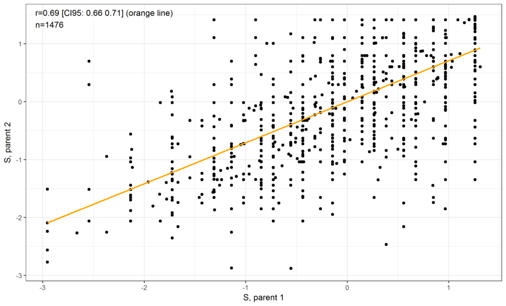
I don’t know any study that actually modeled assortative mating for S as a latent variable, but one can do a crude job at it with the PING data which only has 2 variables for each parent (also has household income which is based on 2 persons and which I ignored). I imputed the missing values which inflated the correlations somewhat (because persons with 1 datapoint get that value for all their variables thus moving correlations towards 1). However, not imputing the values biases the estimate downwards because lower S people are more likely to avoid reporting their income, education etc., so excluding these cases results in reduction of variance and hence observed correlations. If we use the imputed values, the parental S correlation looks like this:
We can see that the measure of S is problematic because there is a ceiling effect at S ≈ 1.25. These are the cases where both parents had the maximum educational and occupation level.
Another assumption is that there is no outcome heritability for the indicators i.e. no heritable group factors for S indicators. In other words, after we can S into account, there will not be any correlations between e.g. educational levels between generations. This is problematic not entirely true, but maybe mostly true. One can modify the model to include paths from the indicators across generations.
In reality land the correlations between GHC and S will not be 1.00 because chance events probably have some effect on the attained S (according to Woody Allen at least). For instance, which education and hence career paths people choose often depend on uncertain/semi-random choices made while young. This would generally bias the observed S~~S relationships downwards. If one relies on aggregate data (e.g. surnames), as Clark does, then it will not be a problem. Clark’s approach will be unbiased if the assumption about no heritable group factors holds.
Related to the above is historically when women did not work outside the home or get educated means that for old data, female S is mostly just a function of their spouse’s S, and thus does not represent their own GHC so strongly as it could.
Grandparent effects, correlations between children’s and grandparents’ S (correlation between blue and red S) will be seen to the extent that there is measurement error in S. Thus, if we are able to form a number of different S’s that can be ranked in quality, the prediction is that the better S estimates will slow smaller grandparent effects than the worse estimates. It’s another instance of controlling for confounding variables is harder than you think.
Clark’s claim about the invariance of the heritability is simply the claim that all the GHC paths will be equal. This can be formally tested in SEM. An implication of this model together with Clark’s assumption of constant heritability is that cross-national or cross-temporal variation seen in correlations between single indicators simply reflect differential S factor loadings for these datasets. This can result from change in the distribution of education which influences the Pearson correlations/OLS estimates.
An interesting prediction can be made from the model: there will be stronger intergenerational relationships for the indicators that have stronger S loadings. I also conjecture that the assortative mating correlations will mirror the S loadings.
Another prediction is that if one has data for 3 generations, and one can identify chance events in generation 2 (green), then these will explain differences between generation 1 and 3 (blue and red). This is because children do not inherit the chance events from their parents and their S will be closer to their GHC. For instance, if there are high S grandparents/blues and low S parents/greens due to some chance event, the children’s/reds’ S will be higher than their parents’ and closer to their grandparents’. Such a chance event could be an infectious disease or a car accident that left the parents crippled and reduced their S.
See also:
- https://westhunt.wordpress.com/2014/03/23/the-son-also-rises/
- https://westhunt.wordpress.com/2014/03/24/simple-mobility-models/
- https://westhunt.wordpress.com/2014/03/29/simple-mobility-models-ii/
- https://jaymans.wordpress.com/2014/03/31/the-son-becomes-the-father/


