Probably the most common objection to studies of polygenic scores for education/intelligence for race differences is that the polygenic scores are less valid for non-European populations. For instance, here’s a recent neat study showcasing this for height:

In this sample, a one standard deviation increase in the polygenic score relates to about a 0.32 standard deviation (about 2 cm) increase in actual height in the British population, slightly less so in the Irish and Polish populations, about 0.25 in Indians, 0.20 in Chinese, and about 0.15 in admixed African-Europeans, all sampled from the UK. But one can go further. Looking inside each individual with mixed ancestry, one can also compute the validity of the polygenic scores derived from the European or African parts of the genome, showing that the validity inside the African part is about 0.12, and about 0.32 inside the British (right side above). The later value is the same as for pure British people.
The same thing is found for polygenic scores for education/intelligence. Here’s a simple result from our 2019 study using the PNC dataset (large American dataset of approx. 12 year olds):
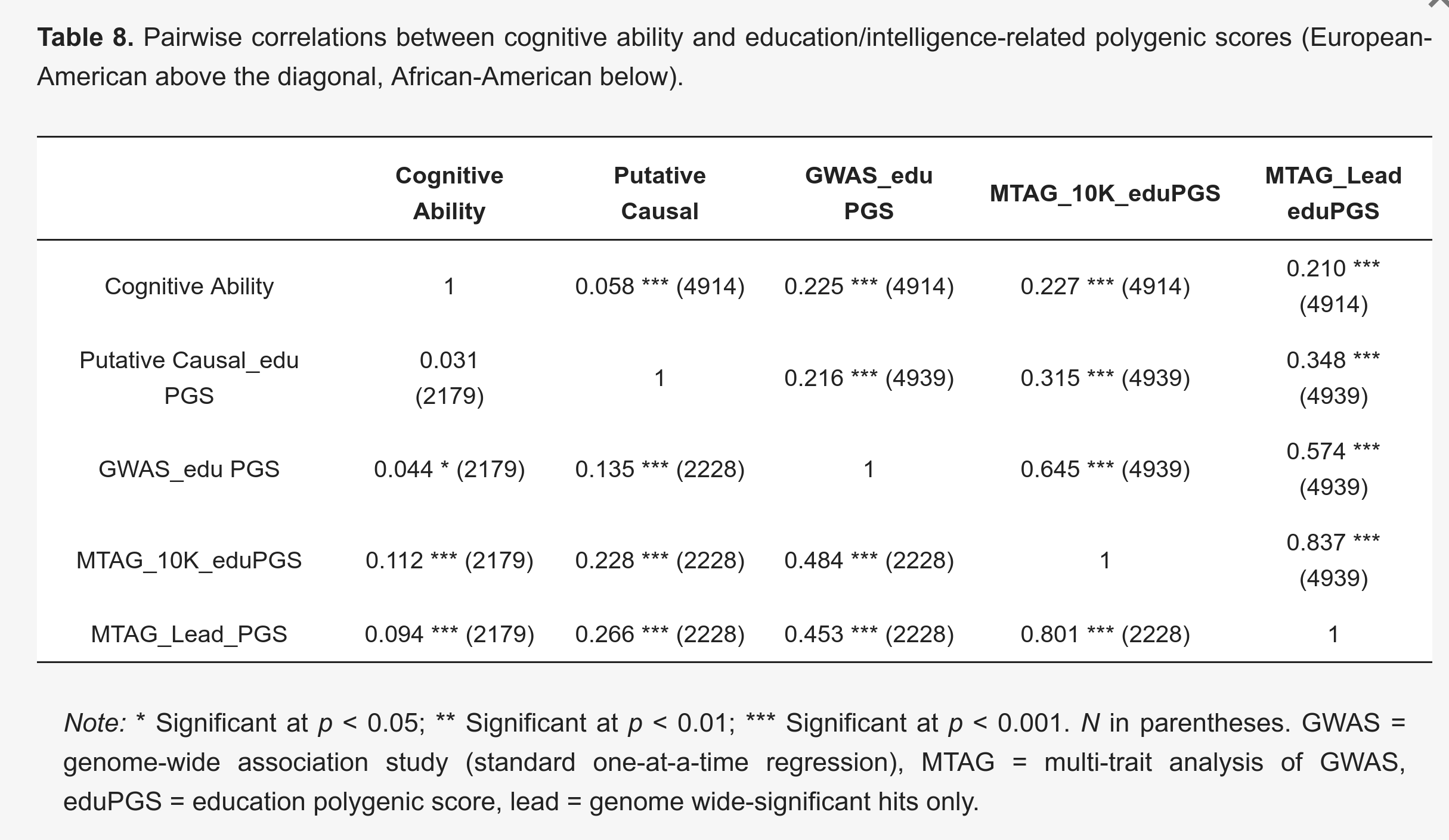
For the MTAG polygenic scores, the validity is roughly twice in American Whites (Europeans) compared to American Blacks (African Americans), about r’s 0.22 vs. 0.10. This is much the same as the case for the height polygenic scores in the UK data above (beta’s 0.32 vs. 0.15).
Is this a problem for comparing the group means? Not by itself actually. It depends on the reason why the polygenic scores are less valid. If this is due to having a larger component of random noise, it will NOT affect the rank order of group comparisons. Here’s a simulated example showing this:
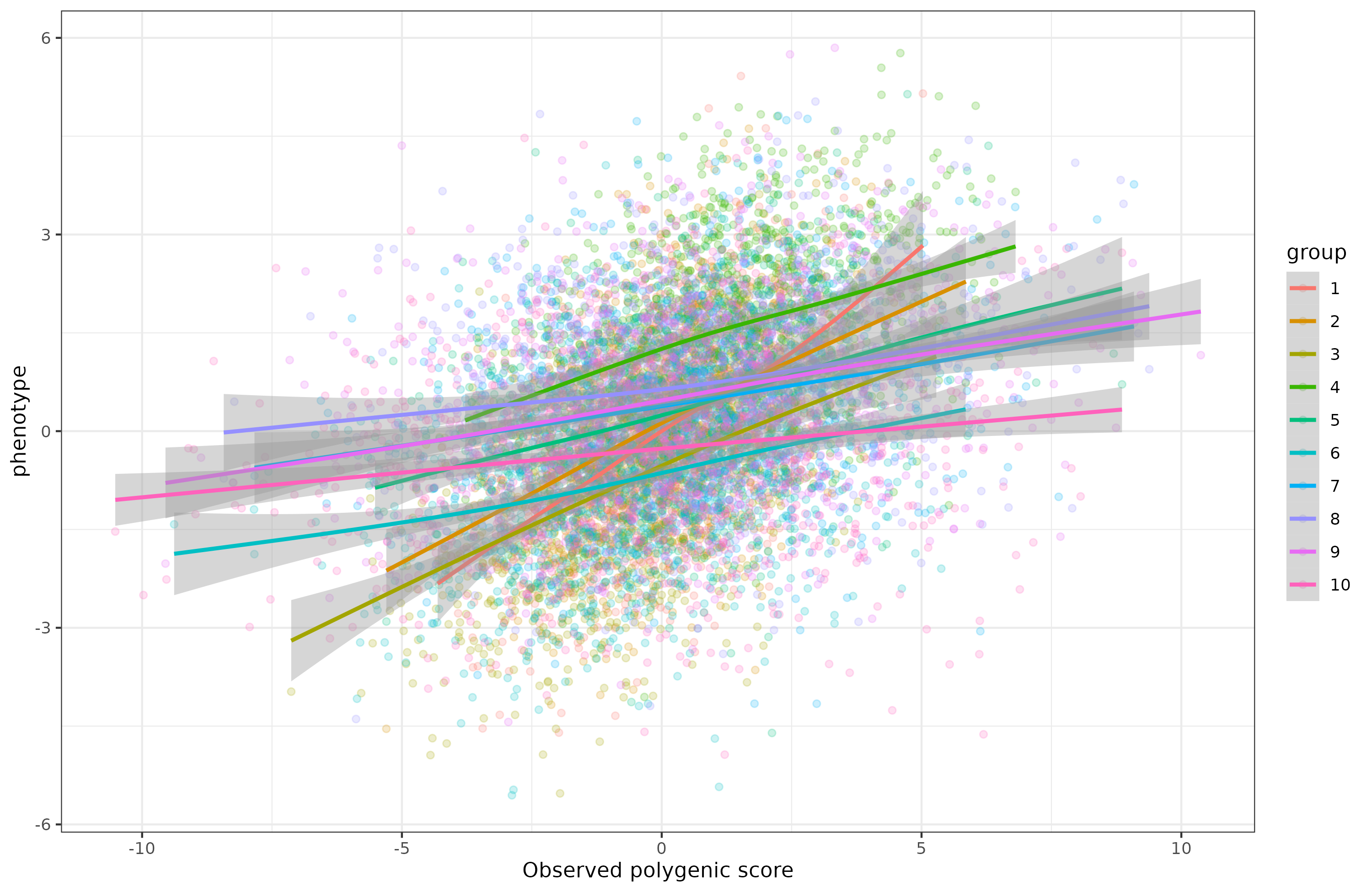
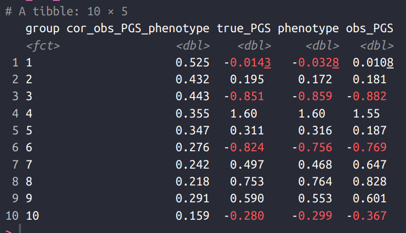
It doesn’t look pretty, the regression lines are all over the place, showing that the polygenic scores are biased predictors (differing in intercept and slope). But biased in what way? Here’s the correlations of the polygenic scores with the phenotype within each group:
In this case, we imagine that we trained a genetic model (“GWAS”) on group 1 (which then has a mean of ~0), and the other groups are increasingly genetically distant from group 1, so the polygenic score falls in validity. That’s why the plot looks like it does, along with the associated group means.
However, when you analyze the data at the group level, this is what it looks like:
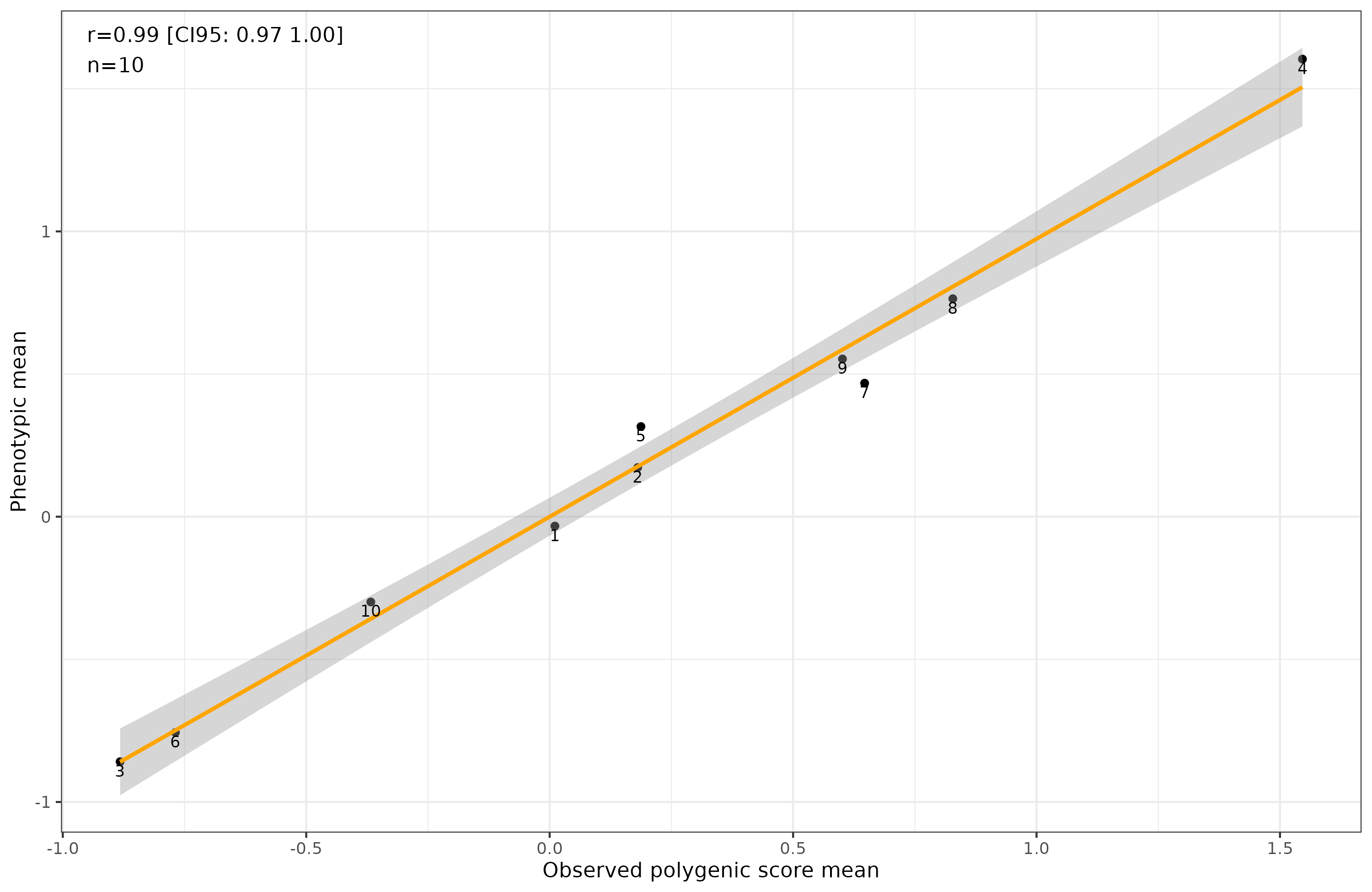
Gone is the bias! Why? Random errors cancel out and don’t affect means. It doesn’t matter in itself that a predictor is less valid for some groups or others, as long as the error variance is centered on 0. The question then becomes: are the errors in polygenic scores centered on 0? That depends on their cause. In the same new paper, we can read:
- Hu, S., Ferreira, L. A., Shi, S., Hellenthal, G., Marchini, J., Lawson, D. J., & Myers, S. R. (2023). Leveraging fine-scale population structure reveals conservation in genetic effect sizes between human populations across a range of human phenotypes. bioRxiv, 2023-08.
An understanding of genetic differences between populations is essential for avoiding confounding in genome-wide association studies (GWAS) and understanding the evolution of human traits. Polygenic risk scores constructed in one group perform poorly in highly genetically-differentiated populations, for reasons which remain controversial. We developed a statistical ancestry inference pipeline able to decompose ancestry both within and between countries, and applied it to the UK Biobank data. This identifies fine-scale patterns of genetic relatedness not captured by standard and widely used principal components (PCs), and allows fine-scale population stratification correction that removes both false positive and false negative associations for traits with geographic correlations. We also develop and apply ANCHOR, an approach leveraging segments of distinct ancestries within individuals to estimate similarity in underlying causal effect sizes between groups, using an existing PGS. Applying ANCHOR to >8000 people of mixed African and European ancestry, we demonstrate that estimated causal effect sizes are highly similar across these ancestries for 26 of 29 quantitative molecular and non-molecular phenotypes (mean correlation 0.98 +/- 0.08), providing evidence that gene-environment and gene-gene interactions do not play major roles in the poor prediction of European-ancestry PRS scores in African populations for these traits, contradicting previous findings. Instead our results provide optimism that shared causal mutations operate similarly in different groups, focussing the challenge of improving GWAS “portability” between groups on joint fine-mapping.
In other words, they did as explained above. They computed the validity of polygenic scores inside admixed peoples with varying amounts of European ancestry. Inside each of the European parts of the genome, the polygenic scores were equally valid to within 100% Europeans. That means the polygenic scores’ validity is NOT affected by various gene-environment or gene-gene interactions that one might hypothesize or ad hoc claim. Rather, as the authors note, the reason the polygenic scores are less valid for non-European ancestries is that:
LD [linkage disequilibrium] is the most likely source of differences between groups, and potentially the way it is handled creates differences between studies. We showed that while African-ancestry segments show similar predictive power in all individuals, their power is hugely reduced by approximately 3-fold relative to European ancestry segments: approximately a 3-fold reduction in the increase in trait per unit increase in PGS, remarkably consistently across traits (Figure 4e). Our (ρ=1) simulations constructing PGS as for the real data show PGS coefficient estimates resembling the real data for European segments, but a more modest relative reduction (<2-fold for traits with >100 causal markers) for African-ancestry segments. Recent work 14 examining correlations within admixed UKB individuals infers identical causal effect sizes for the African-ancestry and European-ancestry variants, indicating that the 3-fold drop we see is likely the result of reduced tagging of causal variants by the PGS in African ancestry regions, and providing evidence against e.g. local interactions among clustered causal variants altering effect sizes. If, for example, selection against trait-impacting variants59,60 results in larger frequency differences for true causal variants between populations than the randomly selected variants used in our simulations, this could explain the observed strong drop-off between groups. ANCHOR might be applied to groups outside the UK, for example African-Americans 14 , that show similar admixture patterns. Resolution for individual traits is expected to grow greatly as sample sizes in such populations improve in coming years.
Linkage disequilibrium (LD) is the technical term for when genetic variants are correlated due to shared descent. In more understandable terms, it’s when the variants are close on the genome, so that they tend to be inherited together during recombination. Recombination is the random shuffling around of genetic material that happens when you produce gametes, i.e., sex cells (sperm and eggs). These kinds of cells only have 1 copy of each chromosome (haploid). But they don’t just have one of the originator’s two chromosomes in full. Instead different parts of a given chromosome are combined to become the new version of that chromosome that is found in those cells. Races that split many 1000s year ago have different histories of how genetic variants got shuffled around in this way, and so the correlations between specific genetic variants will be somewhat different. Correlations between variants are the strongest for populations that have the smallest effective population size, and the weakest for those that have a large effective population size. Thus, races that underwent from recent bottlenecks (e.g. Ashkenazi Jews, Finns, French Canadians) have very strong correlations (LD) among their genetic variants, and those that didn’t experience such strong bottlenecks have weak correlations (Africans). What this means in practice is that when you train a genetic model on Europeans (who experienced the out of Africa bottleneck, and some others later), their variants will be moderately strongly correlated. When you find that genetic variant G1 predicts height, it is not generally because that variant itself is causal for height. Rather, it just happens to be close on the genome to a causal variant which it is correlated with. Thus, when you take this genetic model you have trained on Europeans and apply it to some other groups, the degree to which the variants you are using to predict correlate with the true causal variants will be somewhat weaker on average. The reason for the correlations generally being weaker is that the variants your model picked in the European dataset to proxy (stand in for) the causal variant(s) are the strongest proxies in that population. They won’t be on average in the other populations (winner’s curse, of sorts). Based on this, you get the prediction that the more distant a race is from the European training sample, the less well the polygenic scores due to the different and weaker correlations between proxy variants and causal variants. This is called LD-decay (LDD). So they will work the worst on Africans (the most distant group, out of Africa split 70k+ years ago), and better on races with recent shared ancestry (e.g. Indians who also have Indo-European ancestry, about 4k years ago), somewhat less well on Northeast Asians (shared Eurasian ancestry, from 50k years ago).
Since the process in which these correlations become better or worse is random due to recombination, the errors that are introduced should also be random with regards to the direction of effect of some allele (an allele is one of the versions that may be found at some locus in the genome, say T vs. T, or ATA vs. ATT). Thus, whether a given allele has a positive or negative effect on some phenotype shouldn’t be related to how well the proxy works across populations. For the polygenic scores to become biased with regards to the means then, the differences in LD between populations have to be somehow correlated with the direction of the alleles for the purposes of some group comparison. There is no plausible way this can happen as far as I know. Davide Piffer (2021) developed a method to check for this possibility. The idea is simple enough. For each genetic variant in a genetic model (in the GWAS), check how strongly it is correlated with other nearby variants in Europeans, and then check the same thing in the other group. This gives you two correlation matrices, which you can then compare for similarity. To the extent that they deviate from identity, the variant’s proxying ability for the causal variant(s) will differ. Thus, for each variant in the genetic model (there might be a few hundred or few thousand), one computes this LD-decay score, and then relates this to the directional frequency gaps between the populations (the effect of focus allele multiplied by the group group in its frequency). Any correlation between LD-decay and the direction of effects suggests that LD-decay is biasing the comparison of the group means. Here’s the results for the African and European data from 1000 genomes for the education genetic predictor:
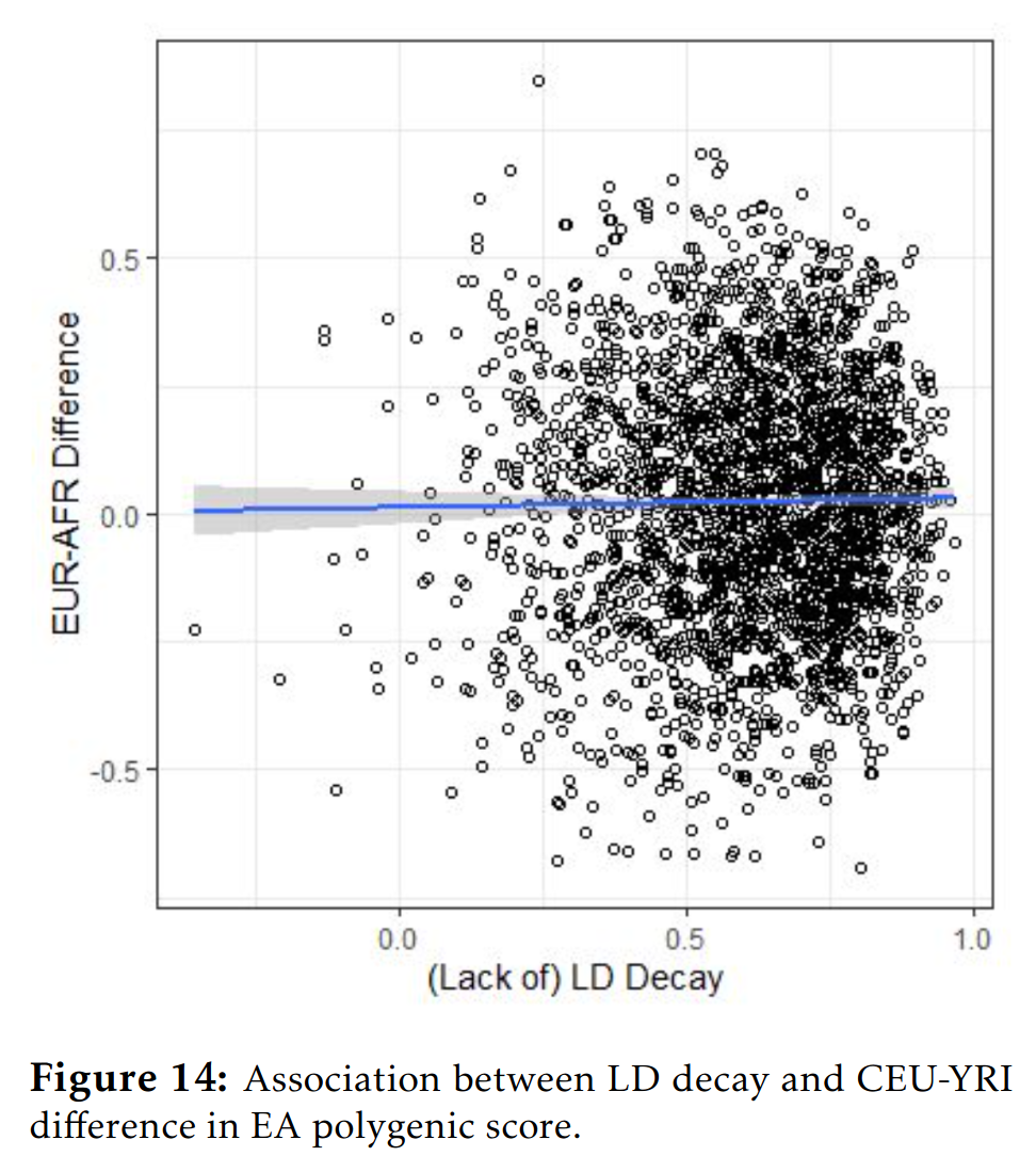
There is no association. In other words, whether a given genetic variant favors Europeans for education (i.e. predicts a higher value for Europeans because the variant is more common in Europeans with a positive allele, or less common with a negative allele), is not related to whether the variant’s proxying ability works the same way (r = 0.015, p = 0.45). Strangely, in some other comparisons, there were correlations of the kind:

Dealing with this LD-decay bias can then be done by predicting what the gap would be at a correlation of 1.00 between the LD patterns i.e., end of the blue line. In this case, it appears that the genetic model favors Europeans for some unknown reason with regards to the LD-decay, whereas the above plot with education didn’t show any bias. Davide is currently working on a large-scale application of this method to various group differences in polygenic scores to see the degree to which they show this kind of bias. In the above versions of the plots, the frequency differences were not weighted by the allele betas unfortunately. But in the upcoming studies, they are. Using this approach, one can compute an LD-decay bias corrected score, to avoid this potential bias in studies. In fact, in the EA4 (latest public genomic model for education), the Europeans are now higher than East Asians, which runs counter to the phenotypic data. Using the correction method reverses this bias. The question is how this biased was introduced in the first place? Some kind of uncorrected ancestry confounding in the training data? Problems with microarrays (ascertainment bias)? Something else? I don’t know.
Take-away
- Polygenic scores usually differ in predictive validity (correlation) between races/populations.
- This does not itself mean that group comparisons are invalid.
- There are methods being developed for dealing with at least some of the biases, when they arise.
- Overall averages from polygenic scores are still in line with phenotypic gaps and hereditarian expectations.