Blog

Background
Populations worldwide are aging. Cognitive decline is an important precursor of dementia, illness and death and, even within the normal range, is associated with poorer performance on everyday tasks. However, the impact of age on cognitive function does not always receive the attention it deserves.
Methods
We have explored cross-sectional associations of age with five cognitive tests (word recall, verbal fluency, subtraction, number sequence, and numerical problem solving) in a large representative sample of over 40,000 men and women aged 16 to 100 living in the UK.
Results
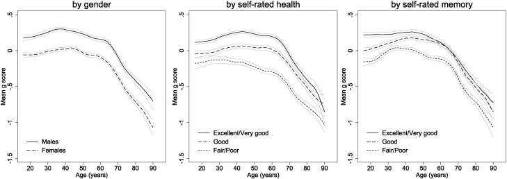
Women performed better on word recall tests and men had higher scores for subtraction, number sequence and numerical problem solving. However, age-cognition associations were generally similar in both genders. Mean word recall and number sequence scores decreased from early adulthood with steeper declines from the mid-60s onwards Verbal fluency, subtraction and numerical problem solving scores remained stable or increased from early to mid-adulthood, followed by approximately linear declines from around age 60. Performance on all tests was progressively lower in respondents with increasingly worse self-rated health and memory. Age-related declines in word recall, verbal fluency and number sequence started earlier in those with the worst self-rated health. There was no compelling evidence for age dedifferentiation (that the general factor of cognitive ability changes in strength with age).
Conclusions
We have confirmed previously observed patterns of cognitive aging using a large representative population sample.

A sample of 40,000? How big were the cognitive ability differences by sex? First, the bare tests, and then the g factor.

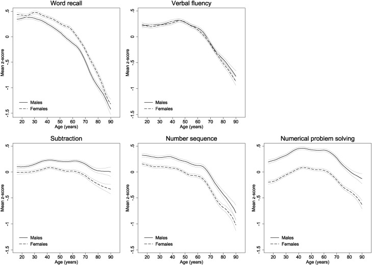
Eye-balling these gives us a gap of about .25 d that seems very stable. But:

We next tested measurement invariance by sex. A multi-group confirmatory factor analysis showed that a model with configural invariance across the sexes had excellent fit to the data (χ2(8) = 283.81, p < 0.001, RMSEA = 0.041, CFI = 0.993, TLI = 0.981), as did a model with weak invariance (χ2(12) = 476.23, p < 0.001, RMSEA = 0.044, CFI = 0.988, TLI = 0.979). However, the model with strong invariance had poorer fit (χ2(17) = 3668.12, p < 0.001, RMSEA = 0.103, CFI = 0.902, TLI = 0.884); indeed, the model with only configural invariance had significantly better fit than either the weak (χ2(4) = 192.42, p < 0.001, ΔAIC = 184.42, ΔBIC = 149.96) or strong (χ2(11) = 3384.32, p < 0.001, ΔAIC = 3366.32, ΔBIC = 3288.78) invariance models. Thus, there was evidence that the g-factor of cognitive ability had different structure across the sexes.

In human language, what does this mean? We have to remember what measurement invariance is. I quote from Alexander Beaujean‘s textbook:

1. Configural. This is the most basic level, and just indicates that LVMs have the same structure in all the groups. That is, the groups have the same number of LVs, formed by the same number of indicator variables, all of which have the same pattern of constrained and estimated parameters. There is no requirement that any estimated coefficients are equal across groups, but the price for these weak assumptions is that there is no reason to believe that the LVs are measuring the same construct in each group. Thus, this level of invariance does not warrant any between-group comparisons of the constructs the LVs represent.

2. Weak. This level adds that, for a given indicator, the loadings are the same across groups. Latent variances are allowed to vary among groups, though. With weak invariance, there is a weak argument that the LVs are equivalent between groups, but, at most, this condition only allows a comparison of the latent variances and covariances.

3. Strong. This level of invariance adds the constraint that, for a given indicator variable, the intercepts are the same among groups. When constraining the intercepts, the latent means are allowed to vary among groups. With this level of invariance, individuals at the same level of a given LV have the same expected value on the indicator variables, irrespective of group membership. Moreover, strong invariance allows for comparisons of the LV. Specifically, latent means, variances, and covariances can all be compared among groups. If there are group differences on strongly-invariant LVs, it likely indicates that there are real difference in these variables, as opposed to the difference being in how the LVs are measured.

4. Strict. This level adds that, for a given indicator, the error variances are constrained to be equal across groups. Usually this level of invariance is not required for making cross-group comparisons of the LVs. Because the error terms in a LVM are comprised of random error variance as well as indicator-specific variance, there is not necessarily the expectation that they would be the same among the groups. Thus, this form of invariance is usually tested, in conjunction with evaluating invariance of the latent variances (level 5), when the area of interest is the reliability of the construct the LV represents. If the latent variances are invariant among the groups, then evaluating strict invariance is really an investigation of construct reliability invariance.

5. Homogeneity of Latent Variable Variances. The variance of a LV represents its dispersion, and thus represents how much variability there is in the construct that the LV represents varies within groups. If there is homogeneity of the latent variances, this indicates the groups used equivalent ranges of the construct for the indicator variables’ values. If this does not hold, however, this indicates that the group with the smaller amount of latent variance is using a narrower range of the construct than the group with the larger amount. Evaluating homogeneity of latent covarinaces can be done, too, but there is usually not much to be gained from such an analysis.

6. Homogeneity of Factor Means. This level of invariance indicates no differences among groups in the average level of the construct the LV represents. Like the more traditional analyses of mean differences (e.g., ANOVA), if there is more than one group then the test of a latent variable’s mean differences usually begins with an omnibus test that constrains the means to be equal across all groups. If this model does not fit the data well, then subsequent tests may be conducted to isolate specific group differences.

Latent variable models (with reflective factors at least) work by positing an unobserved variable (latent, factor) that account for the observed relationships between tests. In this case, we only have 5 tests and we posit a g factor to account for their intercorrelations. In this setting, what it means to say that strong measurement variance fails is to say that when we regress (try to predict) the test scores on our tests from the score on the posited g factor, is that the intercepts in the regressions are not the same by sex.

My guess is that the intercept bias/invariance has to do with the composition of the battery. There were only 5 tests, and their breakdown was: 3 math, 1 verbal, 1 memory. Women had better memory but there was no difference in verbal fluency (this is a common finding despite what you have been told). So, the problem likely is that the g factor is colored because 60% of the tests were about math, and that men have an advantage on the math group factor. Since the math group factor was not modeled here (and could not due to too few tests), it shows up as intercept bias for the g factor. This is omitted variable bias. This is also present for e.g. SAT, where women get higher GPA than their SAT scores predict. That’s because they have an advantage in personality (conscientiousness/study habits) that isn’t modeled. Simulation here: http://emilkirkegaard.dk/understanding_statistics/?app=test_bias_omitted_variable_bias

In fact, the data for this study are quasi-public. I was able to get them in a few minutes. Not mentioned by the authors is that there are item level data for the cognitive tests. But they didn’t give the same items to everybody, so the data are not easy to analyze (have to analyze subsets with complete data or merge items with assumed equal properties (what the authors did)). For instance, wave 3 (the subset the authors analyze) has 3,022 variables alone. About 400 of these have to do with the cognitive testing. They are not all about whether someone got an item right or wrong, but about things such as whether the interviewer thought that the subject was stressed or anxious during testing. I was able to do some rudimentary analyses to confirm the findings. I only used the subtraction, fluency and numeric ability data because these were easy to work with. They produced a fairly skewed distribution due to lack of difficult items.

The age pattern for the g factor (actually I averaged the z scores using equal weights).

And if we remove age by LOESS:

The standardized difference is .22 d, or 3.3 IQ using this method.

The results present something of a dilemma for the blank slaters. They must either accept that there is a difference in g for a very large sample of mostly UK Whites and that this was almost entirely stable over an age span of 70 years or so. Or they can say that the test has a biased composition and the g biased, and that is correct I think, but this just means that men instead have an advantage in mathematical ability that is just as consistent across the age span as the g one. In fact, men may have both.

The very strong stability of results across such an age span makes the results very hard to explain in terms of unequal education, stereotypes etc. There have been large social changes for women over the last 70 years, but about none observable in the age pattern. Hence, it is unlikely that the difference is due to these changing social factors.

The million dollar question is: How do we square this with results from very large Romanian study? It used good quality tests and had a sample size of 15,000. So, as far as tests go, the Romanian study wins. As far as sample size goes, the British study wins. Perhaps the g difference observed here was entirely due to battery composition. Or perhaps there are cross-population differences in sex differences in cognition (as argued e.g. by Davide Piffer).

For those wondering if the data are useful for country of origin analysis. The answer is no. There are variables for country of origin (good, captures first generation) and mother/father’s country of origin (very good, captures second generation and mixed origins), these variables have almost no data. As in, 200 datapoints for a sample of 60k persons. Maybe I missed something and I will have to take a closer look at a later point (i.e. probably never).