Abstract
Researcher choice in reporting of regression models allow for questionable research practices. Here I present a function for R that reports all possible regression models given a set of predictors and a dependent variable. I illustrate this function on two datasets of artificial data.
Introduction
In an email to L.J Zigerell I wrote:
I had a look at your new paper here: http://rap.sagepub.com/content/2/1/2053168015570996 [Zigerell, 2015]
Generally, I agree about the problem. Pre-registration or always reporting all comparisons are the obvious solutions. Personally, I will try to pre-register all my survey-type studies from now on. The second is problematic in that there are sometimes quite a lot of ways to test a given hypothesis or estimate an effect with a dataset, your paper mentions a few. In many cases, it may not be easy for the researcher to report all of them by doing the analyses manually. I see two solutions: 1) tools for making automatic comparisons of all test methods, and 2) sampling of test methods. The first is preferable if it can be done, and when it cannot, one can fall back to the second. This is not a complete fix because there may be ways to estimate an effect using a dataset that the researcher did not even think of. If the dataset is not open, there is no way for others to conduct such tests. Open data is necessary.
I have one idea for how to make an automatic comparison of all possible ways to analyze data. In your working paper, you report only two regression models (Table 1). One controlling for 3 and one for 6 variables in MR. However, given the choice of these 6 variables, there are 2^6-1 (63) ways to run the MR analysis (the 64th is the empty model, I guess which could be used to estimate the intercept but nothing else). You could have tried all of them, and reported only the ones that gave the result you wanted (in line with the argument in your paper above). I’m not saying you did this of course, but it is possible. There is researcher degree of freedom about which models to report. There is a reason for this too which is that normally people run these models manually and running all 63 models would take a while doing manually (hard coding them or point and click), and they would also take up a lot of space to report if done via the usual table format.
You can perhaps see where I’m going with this. One can make a function that takes as input the dependent variable, the set of independent variables and the dataset, and then returns all the results for all possible ways to include these into MRs. One can then calculate descriptive statistics (mean, median, range, SD) for the effect sizes (std. betas) of the different variables to see how stable they are depending on which other variables are included. This would be a great way to combat the problem of which models to report when using MR, I think. Better, one can plot the results in a visually informative and appealing way.
With a nice interactive figure, one can also make it possible for users to try all of them, or see results for only specific groups of models.
I have now written the code for this. I tested it with two cases, a simple and a complicated one.
Simple case
In the simple case, we have three variables:
a = (normally distributed) noise
b = noise
y = a+b
Then I standardized the data so that betas from regressions are standardized betas. Correlation matrix:
|
a
|
b
|
y
|
|
|
a
|
1.00
|
0.01
|
0.70
|
|
b
|
0.01
|
1.00
|
0.72
|
|
y
|
0.70
|
0.72
|
1.00
|
The small departure from expected values is sampling error (n=1000 in these simulations). The beta matrix is:
|
a
|
b
|
|
|
1
|
0.7
|
NA
|
|
2
|
NA
|
0.72
|
|
3
|
0.7
|
0.71
|
We see the expected results. The correlations alone are the same as their betas together because they are nearly uncorrelated (r=.01) and correlated to y at about the same (r=.70 and .72). The correlations and betas are around .71 because math.
Complicated case
In this case we have 6 predictors some of which are correlated.
a = noise
b = noise
c = noise
d = c+noise
e = a+b+noise
f = .3*a+.7*c+noise
y = .2a+.3b+.5c
Correlation matrix:
|
a
|
b
|
c
|
d
|
e
|
f
|
y
|
|
|
a
|
1.00
|
0.00
|
0.00
|
-0.04
|
0.58
|
0.24
|
0.31
|
|
b
|
0.00
|
1.00
|
0.00
|
-0.05
|
0.57
|
-0.02
|
0.47
|
|
c
|
0.00
|
0.00
|
1.00
|
0.72
|
0.01
|
0.52
|
0.82
|
|
d
|
-0.04
|
-0.05
|
0.72
|
1.00
|
-0.04
|
0.37
|
0.56
|
|
e
|
0.58
|
0.57
|
0.01
|
-0.04
|
1.00
|
0.13
|
0.46
|
|
f
|
0.24
|
-0.02
|
0.52
|
0.37
|
0.13
|
1.00
|
0.50
|
|
y
|
0.31
|
0.47
|
0.82
|
0.56
|
0.46
|
0.50
|
1.00
|
And the beta matrix is:
| model # |
a
|
b
|
c
|
d
|
e
|
f
|
|
1
|
0.31
|
NA
|
NA
|
NA
|
NA
|
NA
|
|
2
|
NA
|
0.47
|
NA
|
NA
|
NA
|
NA
|
|
3
|
NA
|
NA
|
0.82
|
NA
|
NA
|
NA
|
|
4
|
NA
|
NA
|
NA
|
0.56
|
NA
|
NA
|
|
5
|
NA
|
NA
|
NA
|
NA
|
0.46
|
NA
|
|
6
|
NA
|
NA
|
NA
|
NA
|
NA
|
0.50
|
|
7
|
0.31
|
0.47
|
NA
|
NA
|
NA
|
NA
|
|
8
|
0.32
|
NA
|
0.83
|
NA
|
NA
|
NA
|
|
9
|
0.34
|
NA
|
NA
|
0.57
|
NA
|
NA
|
|
10
|
0.07
|
NA
|
NA
|
NA
|
0.41
|
NA
|
|
11
|
0.21
|
NA
|
NA
|
NA
|
NA
|
0.45
|
|
12
|
NA
|
0.47
|
0.83
|
NA
|
NA
|
NA
|
|
13
|
NA
|
0.50
|
NA
|
0.58
|
NA
|
NA
|
|
14
|
NA
|
0.31
|
NA
|
NA
|
0.28
|
NA
|
|
15
|
NA
|
0.48
|
NA
|
NA
|
NA
|
0.51
|
|
16
|
NA
|
NA
|
0.87
|
-0.07
|
NA
|
NA
|
|
17
|
NA
|
NA
|
0.82
|
NA
|
0.45
|
NA
|
|
18
|
NA
|
NA
|
0.78
|
NA
|
NA
|
0.09
|
|
19
|
NA
|
NA
|
NA
|
0.58
|
0.48
|
NA
|
|
20
|
NA
|
NA
|
NA
|
0.43
|
NA
|
0.34
|
|
21
|
NA
|
NA
|
NA
|
NA
|
0.40
|
0.45
|
|
22
|
0.31
|
0.47
|
0.83
|
NA
|
NA
|
NA
|
|
23
|
0.34
|
0.49
|
NA
|
0.59
|
NA
|
NA
|
|
24
|
0.29
|
0.45
|
NA
|
NA
|
0.03
|
NA
|
|
25
|
0.20
|
0.47
|
NA
|
NA
|
NA
|
0.46
|
|
26
|
0.31
|
NA
|
0.86
|
-0.04
|
NA
|
NA
|
|
27
|
0.09
|
NA
|
0.82
|
NA
|
0.40
|
NA
|
|
28
|
0.32
|
NA
|
0.83
|
NA
|
NA
|
-0.01
|
|
29
|
0.09
|
NA
|
NA
|
0.58
|
0.43
|
NA
|
|
30
|
0.27
|
NA
|
NA
|
0.47
|
NA
|
0.26
|
|
31
|
-0.04
|
NA
|
NA
|
NA
|
0.42
|
0.46
|
|
32
|
NA
|
0.47
|
0.84
|
-0.02
|
NA
|
NA
|
|
33
|
NA
|
0.32
|
0.82
|
NA
|
0.27
|
NA
|
|
34
|
NA
|
0.47
|
0.77
|
NA
|
NA
|
0.10
|
|
35
|
NA
|
0.33
|
NA
|
0.59
|
0.30
|
NA
|
|
36
|
NA
|
0.50
|
NA
|
0.45
|
NA
|
0.34
|
|
37
|
NA
|
0.37
|
NA
|
NA
|
0.18
|
0.48
|
|
38
|
NA
|
NA
|
0.84
|
-0.02
|
0.45
|
NA
|
|
39
|
NA
|
NA
|
0.82
|
-0.07
|
NA
|
0.09
|
|
40
|
NA
|
NA
|
0.81
|
NA
|
0.45
|
0.02
|
|
41
|
NA
|
NA
|
NA
|
0.48
|
0.44
|
0.27
|
|
42
|
0.31
|
0.47
|
0.83
|
0.00
|
NA
|
NA
|
|
43
|
0.31
|
0.47
|
0.83
|
NA
|
0.00
|
NA
|
|
44
|
0.31
|
0.47
|
0.83
|
NA
|
NA
|
0.00
|
|
45
|
0.32
|
0.48
|
NA
|
0.59
|
0.02
|
NA
|
|
46
|
0.27
|
0.49
|
NA
|
0.49
|
NA
|
0.26
|
|
47
|
0.18
|
0.46
|
NA
|
NA
|
0.03
|
0.46
|
|
48
|
0.09
|
NA
|
0.83
|
-0.02
|
0.40
|
NA
|
|
49
|
0.32
|
NA
|
0.86
|
-0.04
|
NA
|
-0.01
|
|
50
|
0.09
|
NA
|
0.82
|
NA
|
0.40
|
0.00
|
|
51
|
0.02
|
NA
|
NA
|
0.48
|
0.43
|
0.26
|
|
52
|
NA
|
0.32
|
0.83
|
-0.01
|
0.27
|
NA
|
|
53
|
NA
|
0.47
|
0.79
|
-0.02
|
NA
|
0.10
|
|
54
|
NA
|
0.33
|
0.79
|
NA
|
0.26
|
0.06
|
|
55
|
NA
|
0.36
|
NA
|
0.47
|
0.23
|
0.30
|
|
56
|
NA
|
NA
|
0.83
|
-0.02
|
0.44
|
0.02
|
|
57
|
0.31
|
0.47
|
0.83
|
0.00
|
0.00
|
NA
|
|
58
|
0.31
|
0.47
|
0.83
|
0.00
|
NA
|
0.00
|
|
59
|
0.31
|
0.47
|
0.83
|
NA
|
0.00
|
0.00
|
|
60
|
0.26
|
0.48
|
NA
|
0.49
|
0.02
|
0.26
|
|
61
|
0.09
|
NA
|
0.84
|
-0.02
|
0.40
|
0.00
|
|
62
|
NA
|
0.33
|
0.80
|
-0.01
|
0.26
|
0.06
|
|
63
|
0.31
|
0.47
|
0.83
|
0.00
|
0.00
|
0.00
|
So we see that the full model (model 63) finds that the betas are the same as the correlations while the other second-order variables get betas of 0 altho they have positive correlations with y. In other words, MR is telling us that these variables have zero effect when taking into account a, b and c, and each other — which is true.
By inspecting the matrix, we can see how one can be an unscrupulous researcher by exploiting researcher freedom (Simmons, 2011). If one likes the variable d, one can try all these models (or just a few of them manually), and then selectively report the ones that give strong betas. In this case model 60 looks like a good choice, since it controls for a lot yet still produces a strong beta for the favored variable. Or perhaps choose model 45, in which beta=.59. Then one can plausibly write in the discussion section something like this:
Prior research and initial correlations indicated that d may be a potent explanatory factor of y, r=.56 [significant test statistic]. After controlling for a, b and e, the effect was mostly unchanged, beta=.59 [significant test statistic]. However, after controlling for f as well, the effect was somewhat attenuated but still substantial, beta=.49 [significant test statistic]. The findings thus support theory T about the importance of d in understanding y.
One can play the game the other way too. If one dislikes a, one might focus on the models that find a weak effect of a, such as 31, where the beta is -.04 [non-significant test statistic] when controlling for e and f.
It can also be useful to examine the descriptive statistics of the beta matrix:
|
var
|
#
|
n
|
mean
|
sd
|
median
|
trimmed
|
mad
|
min
|
max
|
range
|
skew
|
kurtosis
|
se
|
|
a
|
1
|
32
|
0.24
|
0.11
|
0.31
|
0.25
|
0.03
|
-0.04
|
0.34
|
0.38
|
-0.96
|
-0.59
|
0.02
|
|
b
|
2
|
32
|
0.44
|
0.06
|
0.47
|
0.45
|
0.01
|
0.31
|
0.50
|
0.19
|
-1.10
|
-0.57
|
0.01
|
|
c
|
3
|
32
|
0.82
|
0.02
|
0.83
|
0.82
|
0.01
|
0.77
|
0.87
|
0.10
|
-0.44
|
0.88
|
0.00
|
|
d
|
4
|
32
|
0.25
|
0.28
|
0.22
|
0.25
|
0.38
|
-0.07
|
0.59
|
0.66
|
0.05
|
-1.98
|
0.05
|
|
e
|
5
|
32
|
0.28
|
0.17
|
0.35
|
0.29
|
0.14
|
0.00
|
0.48
|
0.48
|
-0.59
|
-1.29
|
0.03
|
|
f
|
6
|
32
|
0.21
|
0.19
|
0.18
|
0.20
|
0.26
|
-0.01
|
0.51
|
0.52
|
0.27
|
-1.57
|
0.03
|
The range and sd (standard deviation) are useful as a measure of how the effect size of the variable varies from model to model. We see that among the true causes (a, b, c) the sd and range are smaller than among the ones that are non-causal correlates (d, e, f). Among the true causes, the weaker causes have larger ranges and sds. Perhaps one can find a way to adjust for this to get an effect size independent measure of how much the beta varies from model to model. The mad (median absolute deviation, robust alternative to the sd) looks like a very promising candidate the detecting the true causal variables. It is very low (.01, .01 and .03) for the true causes, and at least 4.67 times larger for the non-causal correlates (.03 and .14).
In any case, I hope to have shown how researchers can use freedom of choice in model choice and reporting to inflate or deflate the effect size of variables they like/dislike. There are two ways to deal with this. Researchers must report all the betas with all available variables in a study (this table can get large, because it is 2^n-1 where n is the number of variables), e.g. using my function or an equivalent function, or better, the data must be available for reanalysis by others.
Source code
The function is available from the psych2 repository at Github. The R code for this paper is available on the Open Science Framework repository.
References
Simmons JP, Nelson LD, Simonsohn U. (2011). False-positive psychology: Undisclosed flexibility in data collection and analysis allows presenting anything as significant. Psychological Science 22(11): 1359–1366.