https://www.goodreads.com/book/show/19823567-quantitative-research-in-linguistics
http://gen.lib.rus.ec/book/index.php?md5=3bb68f8bfea90338ad2efa04569108e2
There are few good things to say about this book. The best thing is on the very first page:
Some things never change: the sun rises in the morning. The sun sets in the evening. A lot of linguists don’t like statistics. I have spent a decade teaching English language and linguistics at various universities, and, invariably, there seems to be a widespread aversion to all things numerical. The most common complaint is that statistics is ‘too difficult’. The fact is, it isn’t. Or at least, it doesn’t need to be.
I laughed out hard in the train when reading this.
Not only do linguists not like numbers, they are not very good with them. This is exemplified with this textbook, which contains so many errors I get tired of writing notes in my PDF file.
By definition, the two approaches of analysis also differ in another respect: qualitative research is inductive, that is, theory is derived from the research results. Qualitative analysis is often used in preliminary studies in order to evaluate the research area. For example, we may want to conduct focus groups and interviews and analyse them qualitatively in order to build a picture of what is going on. We can then use these findings to explore these issues on a larger scale, for example by using a survey, and conduct a quantitative analysis. However, it has to be emphasized that qualitative research is not merely an auxiliary tool to data analysis, but a valuable approach in itself!
Quantitative research, on the other hand, is deductive: based on already known theory we develop hypotheses, which we then try to prove (or disprove) in the course of our empirical investigation. Accordingly, the decision between qualitative and quantitative methodology will have a dramatic impact on how we go about our research. Figures 2.1 and 2.2 outline the deductive and inductive processes graphically.
At the beginning of the quantitative-deductive process stands the hypothesis (or theory). As outlined below, a hypothesis is a statement about a particular aspect of reality, such as ‘the lower the socio-economic class, the more non-standard features a speaker’s language shows’. The hypothesis is based on findings of previous research, and the aim of our study is to prove or disprove it. Based on a precisely formulated hypothesis, or research question, we develop a methodology, that is, a set of instruments which will allow us to measure reality in such a way that the results allow us to prove the hypothesis right or wrong. This also includes the development of adequate analytic tools, which we will use to analyse our data once we have collected it. Throughout this book, I will keep reminding readers that it is paramount that hypothesis/research question and methodological analytical framework must be developed together and form a cohesive and coherent unit. In blunt terms, our data collection methods must enable us to collect data which actually fits our research question, as do our data analysis tools. This will become clearer in the course of this and subsequent chapters. The development of the methodological-analytical framework can be a time-consuming process; especially in complex studies we need to spend considerable time and effort developing a set of reliable and valid (see below) tools.
The author has perhaps heard some summary of Popper’s ideas about the hypothetical deductive method. However, Popper aside, science is very much quantitative and inductive. The entire point of meta-analysis is to obtain good summary effects and to check whether results generalize across contexts (i.e. validity generalization á la Hunter and Schmidt).
But that is not all. He then even gets the standard Popperian view wrong. When we confirm a prediction (we pretend to do so, when there is no pre-registration), we don’t prove the theory. That would be an instance of affirming the consequent.
As for qualitative methods being deductive. That makes little sense. I have taken such classes, they usually involve interviews, which is certainly empirical and inductive.
So, in what situations can (and should) we not use a quantitative but a qualitative method? Remember from above that quantitative research is deductive: we base our question and hypotheses on already existing theories, while qualitative research is deductive and is aimed at developing theories. Qualitative research might come with the advantage of not requiring any maths, but the advantage is only a superficial one: not only do we not have a profound theoretical basis, but we also very often do not know what we get – for inexperienced researchers this can turn into a nightmare.
This passage made me very confused because he used deductive twice by error.
[some generally sensible things about correlation and cause]. In order to be able to speak of a proper causal relationship, our variables must show three characteristics:
- a They must correlate with each other, that is, their values must co-occur in a particular pattern: for example, the older a speaker, the more dialect features you find in their speech (see Chapter Seven).
- b There must be a temporal relationship between the two variables X and Y, that is, Y must occur after X. In our word-recognition example in Section 2.4, this would mean that for speed to have a causal effect on performance, speed must be increased first, and drop in participants’ performance occurs afterwards. If performance decreases before we increase the speed, it is highly unlikely that there is causality between the two variables. The two phenomena just co-occur by sheer coincidence.
- c The relationship between X and Y must not disappear when controlled for a third variable.
It has been said that causation implies correlation, but I think this is not strictly true. Another variable could have a statistical suppressor effect, making the correlation between X and Y disappear.
Furthermore, correlation is a measure of a linear relationship, but causation does could be non-linear and thus show a non-linear statistical pattern.
Finally, (c) is just wrong. For instance, if X causes A, …, Z and Y, and we control for A, …, Z, the correlation between X and Y will greatly diminish or disappear because we are indirectly controlling for X. A brief simulation:
set.seed(1123)
{
N = 1000
d_test = data.frame(X = rnorm(N),
Y = rnorm(N) + X, #X causes Y
A1 = rnorm(N) + X, #and also A1-3
A2 = rnorm(N) + X,
A3 = rnorm(N) + X)
}

cor(d_test)
partial.r(d_test, 1:2, 3:5)
The rXY is .71, but the partial correlation of XY is only .44. If we added enough control variables we could eventually make rXY drop to ~0.
While most people usually consider the first two points when analysing causality between two variables, less experienced researchers (such as undergraduate students) frequently make the mistake to ignore the effect third (and often latent) variables may have on the relationship between X and Y, and take any given outcome for granted. That this can result in serious problems for linguistic research becomes obvious when considering the very nature of language and its users. Any first year linguistics student learns that there are about a dozen sociolinguistic factors alone which influence they way we use language, among them age, gender, social, educational and regional background and so on. And that before we even start thinking about cognitive and psychological aspects. If we investigate the relationship between two variables, how can we be certain that there is not a third (or fourth of fifth) variable influencing whatever we are measuring? In the worst case, latent variables will affect our measure in such a way that it threatens its validity – see below.
This is a minor complaint about language, but I don’t understand why the author calls hidden/missing/omitted variables for latent variables, which has an all together different meaning in statistics!
One step up from ordinal data are variables on interval scales. Again, they allow us to label cases and to put them into a meaningful sequence. However, the differences between individual values are fixed. A typical example are grading systems that evaluate work from A to D, with A being the best and D being the worst mark. The differences between A and B are the same as the difference between B and C and between C and D. In the British university grading system, B, C and D grades (Upper Second, Lower Second and Third Class) all cover a stretch of 10 percentage points and would therefore be interval; however, with First Class grades stretching from 70 to 100 per cent and Fail from 30 downwards, this order is somewhat sabotaged. In their purest form, and in order to avoid problems in statistical analysis, all categories in an interval scale must have the same distance from each other.
This is somewhat unclear. What interval variable really means is that the intervals are equal in meaning. A difference of 10 points means is the same whether it is between IQ 100 and 110, or between 70 and 80. (If you are not convinced that IQ scores are at least approximately interval-scale, read Jensen 1980 chapter 4).
Laws are hypotheses or a set of hypotheses which have been proven correct repeatedly. We may think of the hypothesis: ‘Simple declarative sentences in English have subject-verb-object word order’. If we analyse a sufficient number of simple English declarative sentences, we will find that this hypothesis proves correct repeatedly, hence making it a law. Remember, however, based on the principle of falsifiability of hypotheses, if we are looking at a very large amount of data, we should find at least a few instances where the hypothesis is wrong – the exception to the rule. And here it becomes slightly tricky: since our hypothesis about declarative sentences is a definition, we cannot really prove it wrong. The definition says that declarative sentences must have subject-verb-object (SVO) word order. This implies that a sentence that does not conform to SVO is not a declarative; we cannot prove the hypothesis wrong, as if it is wrong we do not have a declarative sentence. In this sense it is almost tautological. Hence, we have to be very careful when including prescriptive definitions into our hypotheses.
This paragraph mixes up multiple things. Laws can be both statistical and absolute. Perhaps the most commonly referred to laws are Newton’s laws of motion, which turned out to be wrong and thus are not laws at all. They were however thought to be absolute, thus not admitting any counterexamples. Any solid counter-example disproves a universal generalization.
But then he starts discussing falsifiability and how his example hypothesis was not falsifiable, apparently. The initial wording does not make it seem like a definition however.
A few general guidelines apply universally with regard to ethics: first, participants in research must consent to taking part in the study, and should also have the opportunity to withdraw their consent at any time. Surreptitious data collection is, in essence, ‘stealing’ data from someone and is grossly unethical – both in the moral and, increasingly, in the legal sense.
The author is apparently unaware of how any large internet site works. They all gather data from users without explicit consent. It also basically bans data scraping, which is increasingly used in quantitative linguistics.
The probably most popular statistical tool is the arithmetic mean-, most of us will probably know it as the ‘average’ – a term that is, for various reasons we will ignore for the time being, not quite accurate. The mean tells us the ‘average value’ of our data. It is a handy tool to tell us where about our data is approximately located. Plus, it is very easy to calculate – I have heard of people who do this in their head! In order to calculate a reliable and meaningful mean, our data must be on a ratio scale. Think about it: how could we possible calculate the ‘average’ of a nominal variable measuring, for example, respondents’ sex? One is either male or female, so any results along the lines of ‘the average sex of the group is 1.7’ makes no sense whatsoever.
Interval scale is sufficient for calculating means and the like.
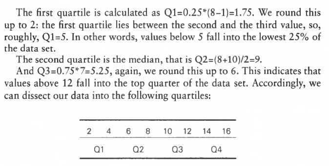
The illustration is wrong. Q2 (median) should be in the middle. Q4 (4*25=100th centile), should be at the end.
A second approach to probabilities is via the relative frequency of an event. We can approximate the probability of a simple event by looking at its relative frequency, that is, how often a particular outcome occurs when the event if repeated multiple times. For example, when we toss a coin multiple times and report the result, the relative frequency of either outcome to occur will gradually approach 0.5 – given that it is an ‘ideal’ coin without any imbalance. Note that it is important to have a very large number of repetitions: if we toss a coin only 3 times, we will inevitably get 2 heads and 1 tail (or vice versa) but we obviously must not conclude that the 2 probability for heads is P(head) = — (0.66). However, if we toss our coin say 1,000 times, we are likely to get something like 520 heads and 480 tails. P(heads) is then 0.52 – much closer to the actual probability of 0.5.
Apparently, the author forgot one can also get 3 of a kind.
Lastly, there may be cases where we are interested in a union event that includes a conditional event. For example, in our Active sample we know that 45% are non-native speakers, that is, P(NNS)=0.4.
Numerical inconsistency.
Excel (or any other software you might use) has hopefully given you a result of p = 0.01492. But how to interpret it? As a guideline, the closer the p-value (of significance level – we will discuss this later) is to zero, the less likely our variables are to be independent. Our p-value is smaller than 0.05, which is a very strong indicator that there is a relationship between type of words produced and comprehension/production. With our result from the chi-test, we can now confidently say that in this particular study, there is a rather strong link between the type of word and the level of production and comprehension. And while this conclusion is not surprising (well, at least not for those familiar with language acquisition), it is a statistically sound one. Which is far better than anecdotal evidence or guessing.
A p value of .01 is not a “very strong indicator”. Furthermore, it is not an effect size measure (although it is probably correlate with effect size). Concluding large effect size (“strong link”) from small p value is a common fallacy.
With the result of our earlier calculations (6.42) and our df (1) we now go to the table of critical values. Since df=l, we look in the first row (the one below the header row). We can see that our 6.42 falls between 3.841 and 6.635. Looking in the header row, we can see that it hence falls between a significance level of 0.05 and 0.01, so our result is significant on a level of 0.05. If you remember, Excel has given us a p value of 0.014 – not quite 0.01, but very close. As before, with p<0.05, we can confidently reject the idea that the variables are independent, but suggest that they are related in some way.
Overconfidence in p-values.
In an ‘ideal’ world, our variables are related in such a way that we can connect all individual points to a straight line. In this case, we speak of a p e r f e c t c o r r e l a t i o n between the two variables. As we can see in Figures 7.1 and 7.2, the world isn’t ideal and the line is not quite straight, so the correlation between age of onset and proficiency is not perfect – although it is rather strong! Before we think about calculating the correlation, we shall consider five basic principles about the correlation of variables:
1 the Pearson correlation coefficient r can have any value between (and including) -1 and 1, that is, -1 < r <, 1.
2 r = 1 indicates a p e r f e c t p o s it iv e c o r r e l a t i o n , that is, the two variables increase in a linear fashion, that is, all data points lie is a straight line – just as if they were plotted with the help of a ruler.
3 r = -1 indicates a p e r f e c t n e g a t iv e c o r r e l a t i o n , that is, while one variable increases, the other decreases, again, linearly.
4 r=0 indicates that the two variables to not correlate at all. That is, there is no relationship between them.
5 The Pearson correlation only works for normally distributed (or ‘parametric’) data (see Chapter Six) which is on a ratio scale (see Chapter Two) – we discuss solutions for non-parametric distributed data in Chapter Nine.
(Ignore the formatting error.)
(4) is wrong. Correlation of 0 does not mean no relationship. It could be non-linear (as also mentioned in (2-3).
We said above that the correlation coefficient does not tell us anything about causality. However, for reasons whose explanations are beyond the scope of this book, if we square the correlation coefficient, that is, multiply it with itself, the so-called R2(R squared) tells us how much the independent variable accounts for the outcome of the dependent variable. In other words, causality can be approximated via R2 (Field 2000: 90). As reported, Johnson and Newport (1991) found that age of onset and L2 proficiency correlate significantly with r = -0.63. In this situation it is clear that //there was indeed causality, it would be age influencing L2 proficiency – and not vice versa. Since we are not provided with any further information or data about third variables, we cannot calculate the partial correlation and have to work with r=-0.63. If we square r, we get -0.6 3 x -0.63 = 0.3969. This can be interpreted in such a way that age of onset can account for about 40 per cent of the variability in L2 acquisition.
This is pretty good, but it also shows us that there must be something else influencing the acquisition process. So, we can only say that age has a comparatively strong influence on proficiency, but we cannot say that is causes it. The furthest we could go with R2 is to argue that if there is causality between age and proficiency, age only causes around 40% ; but to be on the safe side, we should omit any reference to causality altogether.
If you think about it carefully, if age was the one and only variable influencing (or indeed causing) L2 acquisition, the correlation between the two variables should be perfect, that is, r=l (or r= -l) – otherwise we would never get an R2 of 1! In fact, Birdsong and Molis (2001) replicated Johnson and Newport’s earlier (1989) study and concluded that exogenous factors (such as expose and use of the target language) also influence the syntactic development. And with over 60% of variability unaccounted for, there is plenty of space for those other factors!
A very confused text. Does correlation tell us about causality or not? Partially? Correlation of X and Y increases the probability that there is causality between X and Y, but no that much.
Throughout this chapter, I have repeatedly used the concept of significance, but I have yet to provide a reasonable explanation for it. Following the general objectives of this book of being accessible and not to scare off readers mathematically less well versed, I will limit my explanation to a ‘quick and dirty’ definition.
Statistical significance in this context has nothing to do with our results being of particular important – just because Johnson and Newport’s correlation coefficient comes with a significance value of 0.001 does not mean it is automatically groundbreaking research. Significance in statistics refers to the probability of our results being a fluke or not; it shows the likelihood that our result is reliable and has not just occurred through the bizarre constellation of individual numbers. And as such it is very important: when reporting measures such as the Pearson’s r, we must also give the significance value as otherwise our result is meaningless. Imagine an example where we have two variables A and B and three pairs of scores, as below:
[table omitted]
If we calculate the Pearson coefficient, we get r=0.87, this is a rather strong positive relationship. However, if you look at our data more closely, how can we make this statement be reliable? We have only three pairs of scores, and for variable B, two of the three scores are identical (viz. 3), with the third score is only marginally higher. True, the correlation coefficient is strong and positive, but can we really argue that the higher A is the higher is B? With three pairs of scores we have 1 degree of freedom, and if we look up the coefficient in the table of critical values for df=l, we can see that our coefficient is not significant, but quite simply a mathematical fluke.
Statistical significance is based on probability theory: how likely is something to happen or not. Statistical significance is denoted with p, with p fluctuating between zero and 1 inclusive, translating into zero to 100 per cent. The smaller p, the less likely our result is to be a fluke.
For example, for a Pearson correlation we may get r=0.6 and p=0.03. This indicates that the two variables correlate moderately strongly (see above), but it also tells us that the probability of this correlation coefficient occurring by mere chance is only 3%. To turn it round, we can be 97% confident that our r is a reliable measure for the association between the two variables. Accordingly, we might get a result of r=0.98 and p=0.48. Again, we have a very strong relationship; however, in this case the probability that the coefficient is a fluke is 48% – not a very reliable indicator! In this case, we cannot speak of a real relationship between the variables, but the coefficient merely appears as a result of a random constellation of numbers. We have seen a similar issue when discussing two entirely different data sets having the same mean. In linguistics, we are usually looking for significance levels of 0.05 or below (i.e. 95% confidence), although we may want to go as high as p=0.1 (90% confidence). Anything beyond this should make you seriously worried. In the following chapter, we will come across the concept of significance again when we try and test different hypotheses.
Some truth mixed with falsehoods. p values is the probability of getting the result or a more extreme one given the null hypothesis (r=0 in this case). It is not a measure of scientific importance.
It is not a measure of the reliability of finding the value again if we re-do the experiment. That value is much value, depending on statistical power/sample size.
No, a p value >.05 does not imply it was a true negative. It could be a false negative. Especially when sample size is 3!
The interpretation of the result is similar to that of a simple regression: in the first table, the Regression Statistics tell us that our four independent variables in the model can account for 95% of the variability of vitality, that is, the four variables together have a massive impact on vitality. This is not surprising, seeing that vitality is a compound index calculated from those very variables. In fact, the result for R2 should be 100%: with vitality being calculated from the four independent variables, there cannot be any other (latent) variable influencing it! This again reminds us that we are dealing with models – a simplified version of reality. The ANOVA part shows us that the model is highly significant, with p=0.00.
The task of our statistical test, and indeed our entire research, is to prove or disprove HQ. Paradoxically, in reality most of the time we are interested in disproving H0, that is, to show that in fact there is a difference in the use of non-standard forms between socio-economic classes. This is called the alternative hypothesis H, or HA. Hence:
One cannot prove the null hypothesis using NHST. The best one can do with frequentist stats is to show that the confidence interval is very closely around 0.
The most important part for us is the T(F<f) one-tail’ row: it tells us the significance level. Here p=0.23. This tells us that the variances of our two groups are not statistically significantly different; in other words, even though the variance for CG is nominally higher, we can disregard this and assume that the variances are equal. This is important for our choice of t-test.
I seem to recall that the test approach to t-tests is problematic and that it is better to just always use the robust test. I don’t recall the source tho.
Is this really sufficient information to argue that the stimulus ‘knowledge activation’ results in better performance? If you spend a minute or so thinking about it, you will realise that we have only compared the two post-test scores. It does not actually tell us how the stimulus influenced the result. Sadighi and Zare have also compared the pre-test scores of both groups and found no significant difference. That is, both groups were at the same proficiency level before the stimulus was introduced. Yet, we still need a decent measure that tells us the actual change that occurs between EG and CG, o rather: within EG and CG. And this is where the dependent t-test comes into play.
Another instance of p > alpha ergo no differences fallacy.
The really interesting table is the second one, especially the three rightmost columns labelled F, P-value and Fcrit. We see straightaway that the p-value of p=0.25 is larger than p – 0.05, our required significance level. Like the interpretation of the t-test, we use this to conclude that there is no significant difference in means between the treatment groups. The means may look different, but statistically, they are not. In yet other words, the different type of treatment our students receive does not result in different performance.
Same as above, but note that the author got it right in the very first sentence!
As with most things in research, there are various ways of conducting statistical meta-analyses. I will discuss here the method developed by Hunter and Schmidt (for a book-length discussion, see Hunter and Schmidt 2004: – not for the faint-hearted!). The Hunter-Schmidt method uses the Pearson correlation coefficient r as the effect size. If the studies in your pool do not use r (and quite a few don’t), you can convert other effect sizes into r – see, for example, Field and Wright (2006). Hunter and Schmidt base their method on the assumption of random effect sizes – it assumes that different populations have different effect sizes.
Given the number of errors, I was not expecting to see a reference to that book! Even if the author is mathematically incompetent, he gets the good stuff right. :P
Our true effect size of r= -0.68 lies between these boundaries, so we can consider the result to be significant at a 95% confidence level. So, overall, we can say that our meta-analysis of the AoO debate indicated that there is indeed a strong negative correlation between age of onset and attainment, and that this relationship is statistically significant.
That’s not how confidence intervals work…