Blog

Abstract
A factor analysis was carried out on 6 socioeconomic variables for 506 census tracts of Boston. An S factor was found with positive loadings for median value of owner-occupied homes and average number of rooms in these; negative loadings for crime rate, pupil-teacher ratio, NOx pollution, and the proportion of the population of ‘lower status’. The S factor scores were negatively correlated with the estimated proportion of African Americans in the tracts r = -.36 [CI95 -0.43; -0.28]. This estimate was biased downwards due to data error that could not be corrected for.

Introduction
The general socioeconomic factor (s/S¹) is a similar construct to that of general cognitive ability (GCA; g factor, intelligence, etc., (Gottfredson, 2002; Jensen, 1998). For ability data, it has been repeatedly found that performance on any cognitive test is positively related to performance on any other test, no matter which format (pen pencil, read aloud, computerized), and type (verbal, spatial, mathematical, figural, or reaction time-based) has been tried. The S factor is similar. It has been repeatedly found that desirable socioeconomic outcomes tend are positively related to other desirable socioeconomic outcomes, and undesirable outcomes positively related to other undesirable outcomes. When this pattern is found, one can extract a general factor such that the desirable outcomes have positive loadings and then undesirable outcomes have negative loadings. In a sense, this is the latent factor that underlies the frequently used term “socioeconomic status” except that it is broader and not just restricted to income, occupation and educational attainment, but also includes e.g. crime and health.

So far, S factors have been found for country-level (Kirkegaard, 2014b), state/regional-level (e.g. Kirkegaard, 2015), country of origin-level for immigrant groups (Kirkegaard, 2014a) and first name-level data (Kirkegaard & Tranberg, In preparation). The S factors found have not always been strictly general in the sense that sometimes an indicator loads in the ‘wrong direction’, meaning that either an undesirable variable loads positively (typically crime rates), or a desirable outcome loads negatively. These findings should not be seen as outliers to be explained away, but rather to be explained in some coherent fashion. For instance, crime rates may load positively despite crime being undesirable because the justice system may be better in the higher S states, or because of urbanicity tends to create crime and urbanicity usually has a positive loading. To understand why some indicators sometimes load in the wrong direction, it is important to examine data at many levels. This paper extends the S factor to a new level, that of census tracts in the US.

Data source
While taking a video course on statistical learning based on James, Witten, Hastie, & Tibshirani (2013), I noted that a dataset used as an example would be useful for an S factor analysis. The dataset concerns 506 census tracts of Boston and includes the following variables (Harrison & Rubinfeld, 1978):

• Median value of owner-occupied homes
• Average number of rooms in owner units.
• Proportion of owner units built before 1940.
• Proportion of the population that is ‘lower status’. “Proportion of adults without, some high school education and proportion of male workers classified as laborers)”.
• Crime rate.
• Proportion of residential land zoned for lots greater than 25k square feet.
• Proportion of nonretail business acres.
• Full value property tax rate.
• Pupil-teacher ratios for schools.
• Whether the tract bounds the Charles River.
• Weighted distance to five employment centers in the Boston region.
• Index of accessibility to radial highways.
• Nitrogen oxide concentration. A measure of air pollution.
• Proportion of African Americans.

See the original paper for a more detailed description of the variables.

This dataset has become very popular as a demonstration dataset in machine learning and statistics which shows the benefits of data sharing (Wicherts & Bakker, 2012). As Gilley & Pace (1996) note “Essentially, a cottage industry has sprung up around using these data to examine alternative statistical techniques.”. However, as they re-checked the data, they found a number of errors. The corrected data can be downloaded here, which is the dataset used for this analysis.

The proportion of African Americans
The variable concerning African Americans have been transformed by the following formula: 1000(x – .63)². Because one has to take the square root to reverse the effect of taking the square, some information is lost. For example, if we begin with the dataset {2, -2, 2, 2, -2, -2} and take the square of these and get {4, 4, 4, 4, 4, 4}, it is impossible someone to reverse this transformation and get the original because they cannot tell whether 4 results from -2 or 2 being squared.

In case of the actual data, the distribution is shown in Figure 1.

Figure 1: Transformed data for the proportion of blacks by census tract.

Due to the transformation, the values around 400 actually mean that the proportion of blacks is around 0. The function for back-transforming the values is shown in Figure 2.

Figure 2: The transformation function.

We can now see the problem of back-transforming the data. If the transformed data contains a value between 0 and about 140, then we cannot tell which original value was with certainty. For instance, a transformed value of 100 might correspond to an original proportion of .31 or .95.

To get a feel for the data, one can use the Racial Dot Map explorer and look at Boston. Figure 3 shows the Boston area color-coded by racial groups.

Figure 3: Racial dot map of Boston area.

As can be seen, the races tend to live rather separate with large areas dominated by one group. From looking at it, it seems that Whites and Asians mix more with each other than with the other groups, and that African Americans and Hispanics do the same. One might expect this result based on the groups’ relative differences in S factor and GCA (Fuerst, 2014). Still, this should be examined by numerical analysis, a task which is left for another investigation.

Still, we are left with the problem of how to back-transform the data. The conservative choice is to use only the left side of the function. This is conservative because any proportion above .63 will get back-transformed to a lower value. E.g. .80 will become .46, a serious error. This is the method used for this analysis.

Factor analysis
Of the variables in the dataset, there is the question of which to use for S factor analysis. In general when doing these analyses, I have sought to include variables that measure something socioeconomically important and which is not strongly influenced by the local natural environment. For instance, the dummy variable concerning the River Charles fails on both counts. I chose the following subset:

• Median value of owner-occupied homes
• Average number of rooms in owner units.
• Proportion of the population that is ‘lower status’.
• Crime rate.
• Pupil-teacher ratios for schools.
• Nitrogen oxide concentration. A measure of air pollution.

Which concern important but different things. Figure 4 shows the loadings plot for the factor analysis (reversed).²

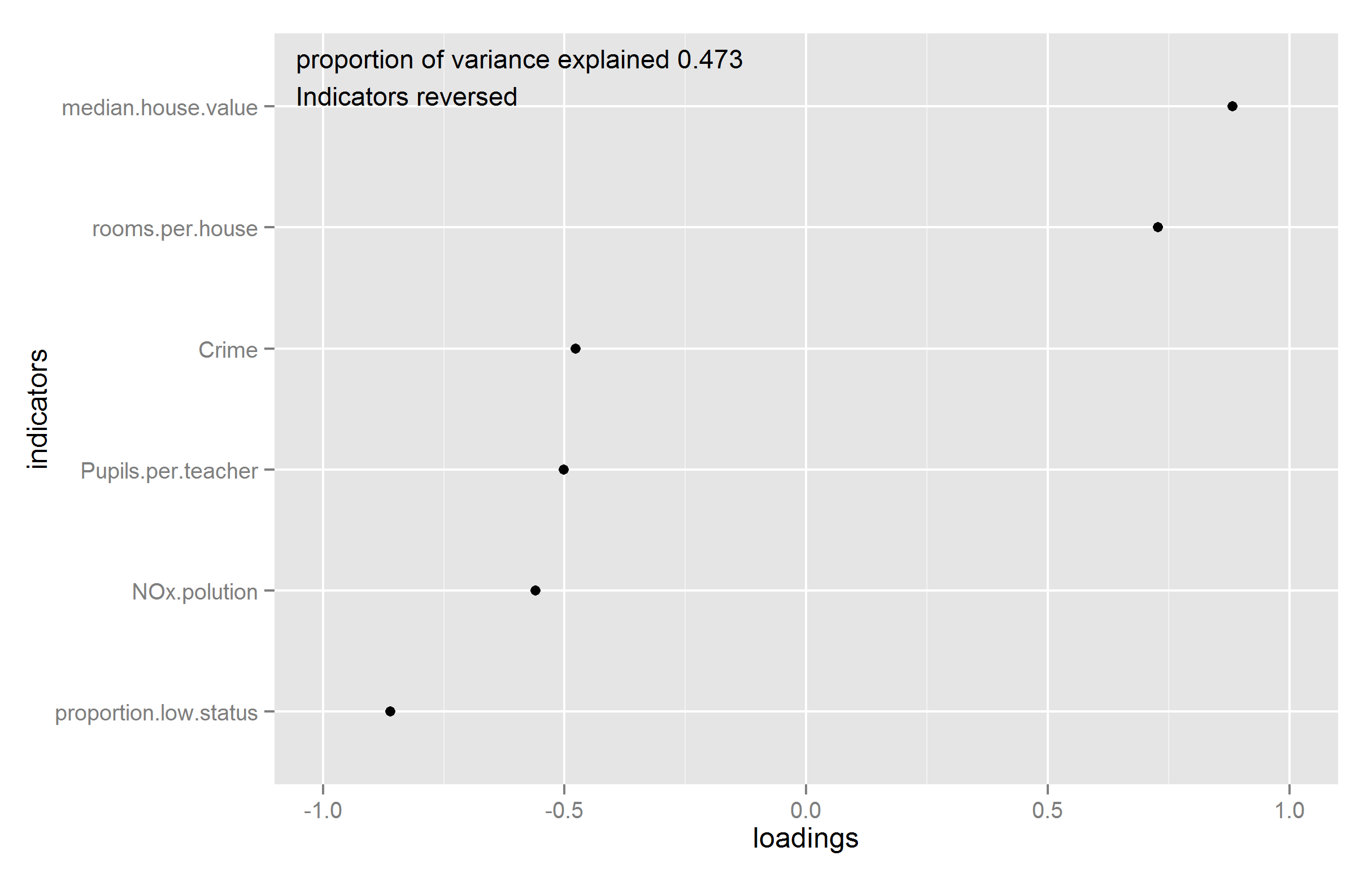
Figure 4: Loadings plot for the S factor.

The S factor was confirmed for this data without exceptions, in that all indicator variables loaded in the expected direction. The factor was moderately strong, accounting for 47% of the variance.

Relationship between S factor and proportions of African Americans
Figure 5 shows a scatter plot of the relationship between the back-transformed proportion of African Americans and the S factor.

Figure 5: Scatter plot of S scores and the back-transformed proportion of African Americans by census tract in Boston.

We see that there is a wide variation in S factor even among tracts with no or very few African Americans. These low S scores may be due to Hispanics or simply reflect the wide variation within Whites (there few Asians back then). The correlation between proportion of African Americans and S is -.36 [CI95 -0.43; -0.28].

We see that many very low S points lie around S [-3 to -1.5]. Some of these points may actually be census tracts with very high proportions of African Americans that were back-transformed incorrectly.

Discussion
The value of r = -.36 should not be interpreted as an estimate of effect size of ancestry on S factor for census tracts in Boston because the proportions of the other sociological races were not used. A multiple regression or similar method with all sociological races as the predictors is necessary to answer this question. Still, the result above is in the expected direction based on known data concerning the mean GCA of African Americans, and the relationship between GCA and socioeconomic outcomes (Gottfredson, 1997).

Limitations
The back-transformation process likely introduced substantial error in the results.

Data are relatively old and may not reflect reality in Boston as it is now.

Supplementary material
Data, high quality figures and R source code is available at the Open Science Framework repository.

References

• Gilley, O. W., & Pace, R. K. (1996). On the Harrison and Rubinfeld data. Journal of Environmental Economics and Management, 31(3), 403–405.
• Gottfredson, L. S. (1997). Why g matters: The complexity of everyday life. Intelligence, 24(1), 79–132. http://doi.org/10.1016/S0160-2896(97)90014-3
• Gottfredson, L. S. (2002). Where and Why g Matters: Not a Mystery. Human Performance, 15(1-2), 25–46. http://doi.org/10.1080/08959285.2002.9668082
• Harrison, D., & Rubinfeld, D. L. (1978). Hedonic housing prices and the demand for clean air. Journal of Environmental Economics and Management, 5(1), 81–102.
• James, G., Witten, D., Hastie, T., & Tibshirani, R. (Eds.). (2013). An introduction to statistical learning: with applications in R. New York: Springer.
• Jensen, A. R. (1998). The g factor: the science of mental ability. Westport, Conn.: Praeger.
• Kirkegaard, E. O. W. (2014a). Crime, income, educational attainment and employment among immigrant groups in Norway and Finland. Open Differential Psychology. Retrieved from http://openpsych.net/ODP/2014/10/crime-income-educational-attainment-and-employment-among-immigrant-groups-in-norway-and-finland/
• Kirkegaard, E. O. W. (2014b). The international general socioeconomic factor: Factor analyzing international rankings. Open Differential Psychology. Retrieved from http://openpsych.net/ODP/2014/09/the-international-general-socioeconomic-factor-factor-analyzing-international-rankings/
• Fuerst, J. (2014). Ethnic/Race Differences in Aptitude by Generation in the United States: An Exploratory Meta-analysis. Open Differential Psychology. Retrieved from http://openpsych.net/ODP/2014/07/ethnicrace-differences-in-aptitude-by-generation-in-the-united-states-an-exploratory-meta-analysis/
• Kirkegaard, E. O. W., & Tranberg, B. (In preparation). What is a good name? The S factor in Denmark at the name-level. Open Differential Psychology. Retrieved from https://osf.io/t2h9c/
• Kirkegaard, E. O. W. (2015). Examining the S factor in Mexican states. The Winnower. Retrieved from https://thewinnower.com/papers/examining-the-s-factor-in-mexican-states
• Rindermann, H. (2007). The g-factor of international cognitive ability comparisons: the homogeneity of results in PISA, TIMSS, PIRLS and IQ-tests across nations. European Journal of Personality, 21(5), 667–706. http://doi.org/10.1002/per.634
• Wicherts, J. M., & Bakker, M. (2012). Publish (your data) or (let the data) perish! Why not publish your data too? Intelligence, 40(2), 73–76. http://doi.org/10.1016/j.intell.2012.01.004

Footnotes

1 Capital S is used when the data are aggregated, and small s is used when it is individual level data. This follows the nomenclature of (Rindermann, 2007).

2 To say that it is reversed is because the analysis gave positive loadings for undesirable outcomes and negative for desirable outcomes. This is because the analysis includes more indicators of undesirable outcomes and the factor analysis will choose the direction to which most indicators point as the positive one. This can easily be reversed by multiplying with -1.