Medical researchers have noticed that some diseases differ by SIRE (self-identified race/ethnicity) groups which differ by genomic (racial) ancestry. Hence, when genomic measures became available (last 15 years or so), they measured peoples relative proportions of ancestry in mixed populations to see if the diseases would be predictable by ancestry. They were. This establishes with high certainty that the group difference is genetic. Of course, this could be used on other traits such as cognitive ability, personality and socioeconomic outcomes (and it has for the latter, we are doing a meta-analysis).
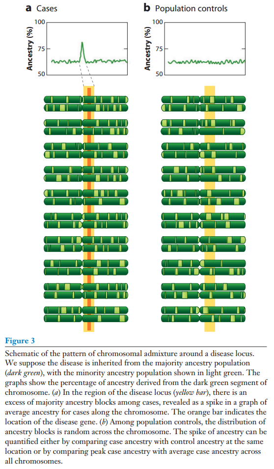
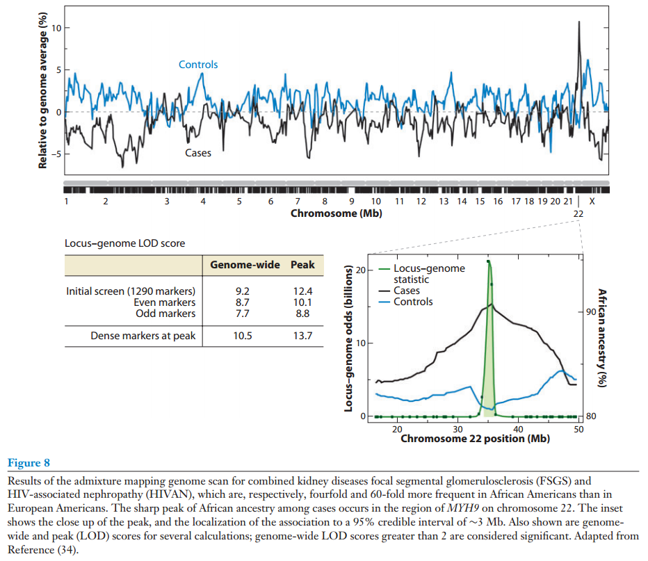
None of this is new. However, here comes the trick. If we know that two ancestries differ for some trait, we can use this to pinpoint where on the genome the genes for this trait are. How? Consider the simple case where we have a disease trait where persons can be clearly scored as either/or (e.g. ever had prostate cancer). We gather a lot of persons with mixed ancestry, cases and controls. Then we look at difference in their ancestry at small intervals of their chromosomes. Because the trait is genetically linked to one ancestry, the cases will show more of the ancestry in some parts of their genome than the controls. These are the places to look for causal variants at. Consider the two figures from Winkler et al 2010.
Winkler, C. A., Nelson, G. W., & Smith, M. W. (2010). Admixture mapping comes of age. Annual review of genomics and human genetics, 11, 65-89.
Winkler reports that the sample sizes needed for this are much smaller than blind-within ancestry standard GWAS (as usually done on Europeans).
This method can be combined with the standard GWAS method. I envision that one ‘simply’ does this by first establishing that a trait differs for genetic reasons across two ancestries in an admixtured group (e.g. African Americans, Hispanics/Mexicans/Mestizos). Then one uses the admixture mapping to establish plausible segments of the genome where causal variants are. This may not be enough to identify specific variants, but one can then use these values as the prior probabilities for a standard GWAS. This should drastically decrease the necessary sample size to find the variants and thus accelerate the search. The faster we can find the variants, the faster we can either edit them directly with CRIPR-like methods or use the information for selection with embryo selection.
This may make it more tractable to find variants when we start doing GWAS on full genomes instead of SNP genomes. SNP genomes have 1e5 to 1e6 variants to examine, but whole genomes have about 3e12, i.e. about 1e6 times more. This means that false positives are an even larger problem. The added statistical power from admixture mapping assisted GWAS should help nicely here.
There is one significant problem with this method, but it is not a scientific one: To use it for a given trait, one must come to terms with the existence of a genetic group difference. It is not surprising that it has primarily been used on disease traits where these claims meet less resistance (because it is about helping). However, a recent mainstream study has examined height and BMI group differences in European populations, so there is some hope that times are a changin.

