Although Meng Hu has recently provided a very thorough review of test bias methods, I thought it would be helpful to have a more visual, intuitive approach for those not inclined to read 30 pages of math methods.
Image some questions on a cognitive test, called items. They can be of any type, vocabulary, spatial rotation, knowledge of pirates in history, it doesn’t matter. Here we will just assume they are generic intelligence items. The goal of what is called item response theory (IRT) is to model the behavior of each item as a function of a small set of parameters. Here I will be using the 2PL model, which has 2 parameters for each item. The abbreviation comes from the idea of the function itself: 2-parameter logistic function. The first parameter is discrimination. This is a value of how strongly the item is related to the construct the test is measuring. Discrimination is the same as the maximum slope of the function, which we will see below. The second parameter is the difficulty, so how hard the item is. You can imagine different mixes of these two parameters, but mathematically, they are unrelated. You can have a difficult item that measures intelligence well, and one that doesn’t. For instance, asking someone what the name of Ludwig van Beethoven’s father is would not be a good test of intelligence, as it’s very specialized knowledge, but it would be a very difficult question. On the other hand, you could give someone a difficult vocabulary question, e.g. what is a cloister?, and this would be a better measure of intelligence.
To illustrate these concepts, I have simulated some data using the mirt R package, and you can see the items plots below:
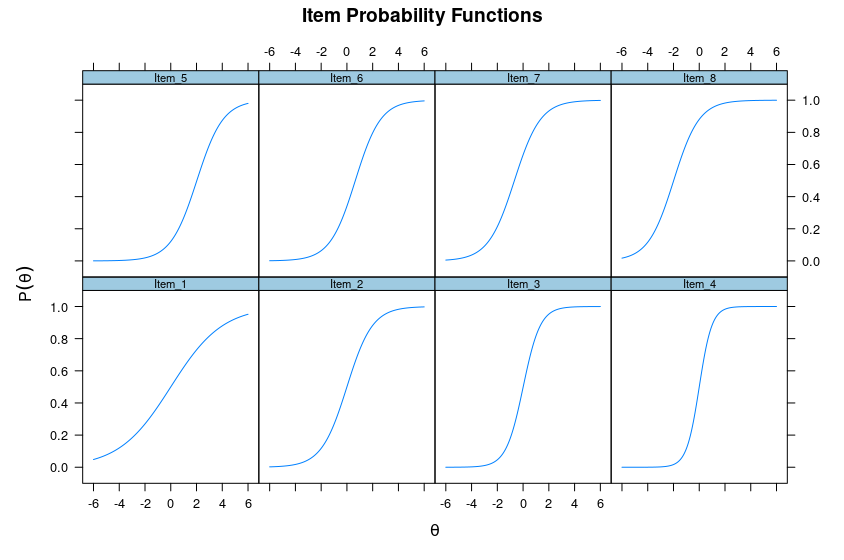
On the X axis is theta which really just refers to the ability of a person taking the item. The Y axis is probability of getting the item right. Naturally, as you see, going from left to right on the X axis increases the probability of getting an item right, no matter the item. This is just the mathematical way of quantifying the commonsense idea that the smarter a person is, the more likely they are to answer some intelligence item correctly.
You will also see that the functions — the lines — differ a bit between the above 8 items. In fact, in the bottom row, the items differ only in their maximum slopes. In this case, the maximum slopes occur at X=theta=0, i.e., that is the center of the 4 items in the bottom row. Clearly, item 4 has a greater slope than item 1, i.e., the value of Y increases faster per increment in X for item 4 than it does for item 1. In other words, item 4 is very good as discriminating between people around ability level 0 (which might be IQ 100), and useless for people far from this value, as they all either get it right 0% of the time or 100% of the item. Item 1 on the other hand, works to measure people’s intelligence across the ability level, but it is comparably poor at this because the difference in chances of getting it right are not so great as with item 4.
Looking now at the top row, there are also 4 items. They have the same shape this time, the same slopes. But notice that their position is displaced along the X axis. Item 5 only reaches 100% probability near X=6, while item 8 reaches this already near X=2. Thus, item 5 is much harder than item 8. That’s difficulty. In numerical terms, here are the item parameters obtained from the data above:

These are the empirical values, but you can see that aside from a bit of sampling error, you can see which values I used to simulate the data. I have also added the factor loading column. The factor loading from traditional factor analysis is in fact equivalent to a transformation of the discrimination/slope parameter. So in this case we see that item 4 is better than item 1, and items 5-8 are equivalent. As we saw in the plots above, the difficulty of the items are the same for items 1-4, but differ between 5-8.
Test bias
With the basics out of the way, we are now ready to ask: what is test bias? Simply, it is when these item parameters are not the same for some groups, or along some continuous variable (e.g. age). When this happens, the items are not functioning the same for the groups, and thus the test might not function equivalently for them. This is called differential item functioning (DIF). But the test might also function without test, it depends on how many items are biased and in which direction. To showcase this, I’ve simulated some more data. Here are the item functions for two groups.

I know, a lot of items, and each by two groups, A and B. Can you spot two items that are definitely not working the same?

That’s right, items 10 and 25. Item 10 shows the B group doing better on the item at any ability level, so item 10 is biased in favor of group B. Item 25, on the other hand, doesn’t appear to measure anything in group B, as the slope is near-zero, even a bit negative. It works fine for group A though. We can then wonder, how do these impact the test itself? First, though, we should look at the distribution of raw scores:

So group B seems to be doing a lot better. We can also look at the factor scores generated from our model (the IRT model):
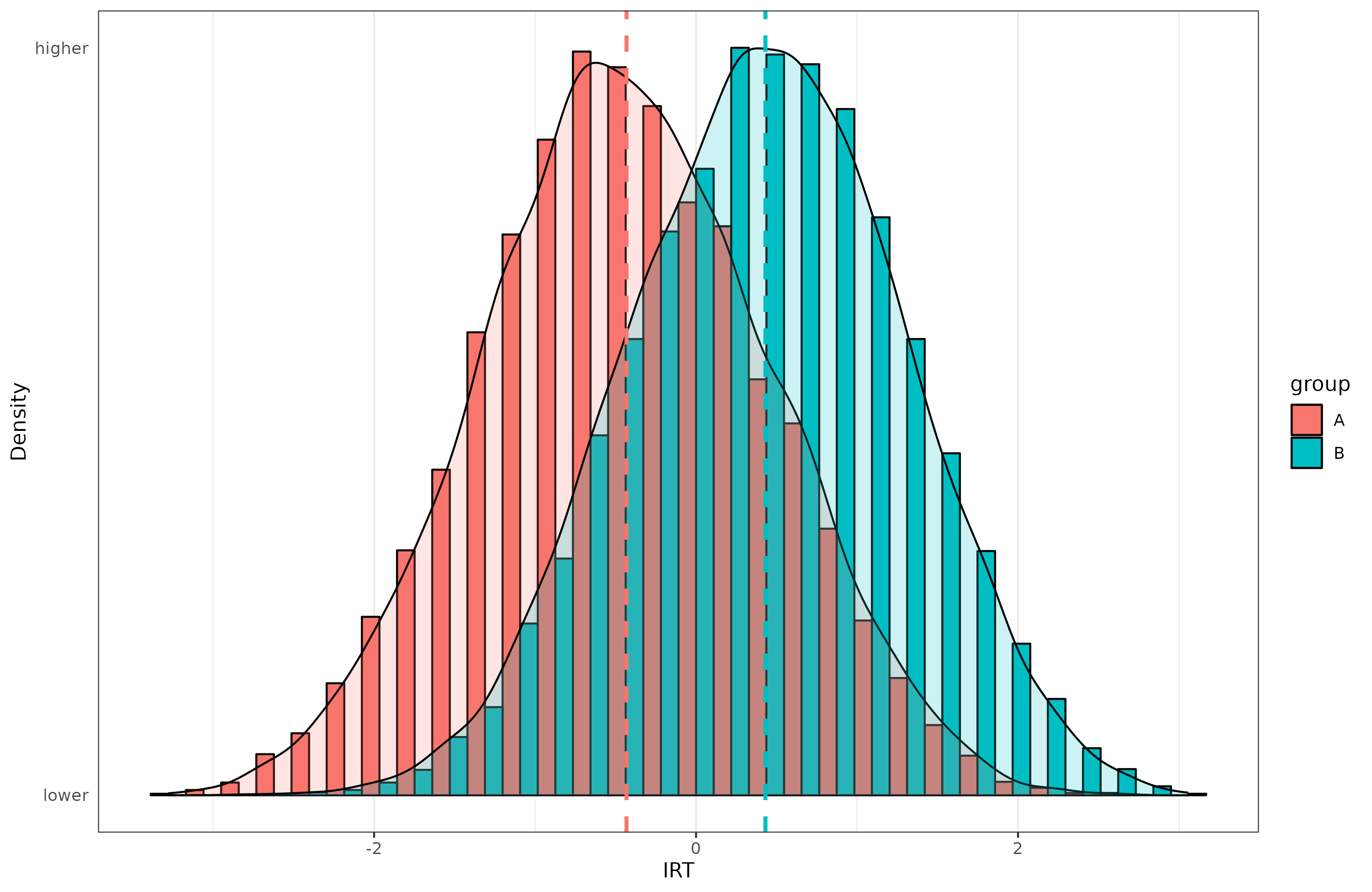
When properly scaled, they look very normal. How big is the gap?
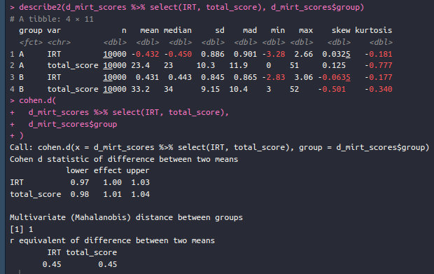
A bit tricky to compute in the head, but in Cohen’s d they are both about 1.00 d, so 15 IQ equivalents in favor of group B. But we also know that there are some biased items, so we can ask: what is the effect of these on the test results? We can plot the total score function by group to assess this:
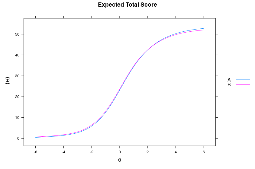
The lines aren’t exactly on top of each other. Below X=0, B’s line is a bit higher, so the test is biased in their favor there. However, after X=2, the blue line is higher, so the test is biased in their favor. Though, over most of the test, it has a slight bias in favor of B. How large is this?

You might be wondering why there are two different versions of each value. For now, just look at conservative and ETSSD. This is the Cohen’s d effect size at the test level of the bias we saw above. The effect size is estimated at 0.034 d, so it is rather trivially biased in favor of group B (the gap we saw was 1.00 d, and we estimate 0.03 bias, so the adjusted gap should be about 0.97). Why the two versions? Because of multiple testing problems. In fact, the analysis produced a bias estimate for each item:

So, we tested all 54 items for bias. Each test produces a p-value for whether bias is present or not. That’s the value in the column called “p”. If you glance over this, you can see that there’s quite a few items that have p-values below 0.05. I count 15 such items. But recall again the plot of each of the 54 items. There only seems to be 2 items with any bias worth caring about. The others are false positives. If we adjust the p-value using bonferroni, we find that there are only 3 biased items: items 10, 25, and 45. In fact, item 45 shows no real bias, and nothing can be seen. It’s just a coincidence, another false positive.
Going back to the table above with results at the test level, the liberal values refer to adjusting for all the items with p < .05 without doing a correction for multiple testing, and conservative refers to only correcting for the items whose p-values survived the multiple testing correction (so 15 vs. 3 items). In this case it hardly matters as the test bias incorrectly found in the false positive items were very small, so the overall effect on the test is tiny according to both standards.
Really, this is just how testing items for bias works in practice. There’s a lot of different methods, but they achieve more or less the same thing as this one. The usual result of such differential item functioning testing is that a few items are found to be biased, but in different directions, and so the test score is not much affected. For instance, in our 2021 study of the vocabulary test at openpsychometrics.org, we found that:
We examined data from the popular free online 45-item “Vocabulary IQ Test” from https://openpsychometrics.org/tests/VIQT/. We used data from native English speakers (n = 9,278). Item response theory analysis (IRT) showed that most items had substantial g-loadings (mean = .59, sd = .22), but that some were problematic (4 items being lower than .25). Nevertheless, we find that using the site’s scoring rules (that include penalty for incorrect answers) give results that correlate very strongly (r = .92) with IRT-derived scores. This is also true when using nominal IRT. The empirical reliability was estimated to be about .90. Median test completion time was 9 minutes (median absolute deviation = 3.5) and was mostly unrelated to the score obtained (r = -.02).
The test scores correlated well with self-reported criterion variables educational attainment (r = .44) and age (r = .40). To examine the test for measurement bias, we employed both Jensen’s method and differential item functioning (DIF) testing. With Jensen’s method, we see strong associations with education (r = .89) and age (r = .88), and less so for sex (r = .32). With differential item functioning, we only tested the sex difference for bias. We find that some items display moderate biases in favor of one sex (13 items had pbonferroni < .05 evidence of bias). However, the item pool contains roughly even numbers of male-favored and female-favored items, so the test level bias is negligible (|d| < 0.05). Overall, the test seems mostly well-constructed, and recommended for use with native English speakers.
We used the above method to the 45 items found in the vocabulary test. The two groups were men and women, all English speakers. WE found 13 items with bias after multiple testing correction. But 7 were biased in favor of men and 6 in favor of women, so it didn’t have any overall effect:

If you count, you can see 7 values on the right side, and 6 on the left. But the mean of this is a trivial pro-male bias below 0.05 d.
I hope this post has helped demystify what test bias really looks like. Remember, if you want more details, dive into Meng Hu’s recent posts. A good textbook on the topic is Christine DeMars’ (2010) Item Response Theory. Oxford University Press.