When I talk science to non-scientists, I often get questions about how to interpret sizes of correlations or other metrics. While one can give rough guidelines invariant of the topic at hand, they can be quite misleading. Most famously, statistician Cohen made up some guidelines decades ago, and while they were based on nothing in particular, they have somehow stuck (like Fisher’s p < .05 threshold). These are:
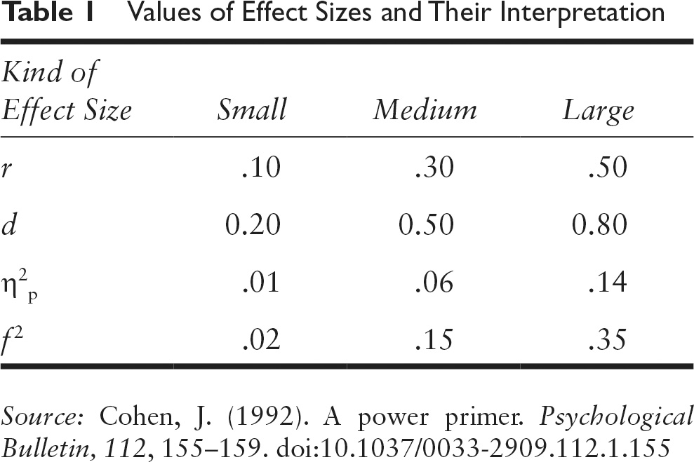
So a correlation of .10 is small, .30 is medium, and .50 is large. Or in Cohen’s d metric (the number of standard deviations between two groups on some metric), 0.20, 0.50, and 0.80. Roughly, you can translate correlations to Cohen’s d in your head because you just need to multiply by 2 for when correlation is far from 1.0. A correlation of 1.00 is an infinitely large d value.
An alternative to the Cohen guidelines is to compare the effect size you are looking at to others reported in the literature. This doesn’t tell you whether it’s large in any natural, real life sense, but whether it’s large relative to others reported in the scientific literature. I have a post compiling a bunch of these empirical effect size reviews. This approach is problematic for reasons that the published effect sizes are unreliable. Often too large due to publication bias and p-hacking, and simultaneously too small due to measurement error that went uncorrected.
You could also opt for a visual impression which you can get from the excellent site by Kristoffer Magnusson (rpsychologist.com). Case in point for Cohen’s d. This metric is very useful in medicine, because it removes the immediate need to understand all sorts of specialist scales used across the fields. For instance, to get an intuitive idea of what a Cohen’s d of 0.50 means, you can look at this:

A Common Language Explanation
With a Cohen’s d of 0.50, 69.1% of the “treatment” group will be above the mean of the “control” group (Cohen’s U3), 80.3% of the two groups will overlap, and there is a 63.8% chance that a person picked at random from the “treatment” group will have a higher score than a person picked at random from the “control” group (probability of superiority). Moreover, in order to have one more favorable outcome in the “treatment” group compared to the “control” group, we need to treat 6.0 people on average. This means that if there are 100 people in each group, and we assume that 20 people have favorable outcomes in the “control” group, then 20 + 16.6 people in the “treatment” group will have favorable outcomes.1
1The values are averages, and it is assumed that 20 (CER) of the “control” group have “favorable outcomes,” i.e., their outcomes are below some cut-off. Change this by pressing the settings symbol to the right of the slider. Go to the formula section for more information.
I would say 0.50 represents quite a nice treatment in medicine. It’s large enough that you can see the effect if you are familiar with a few people taking the treatment. To give a random example. Using minoxidil for male hair loss has an effect size of about 0.50 to 0.80 d according to several meta-analyses.
However, the purpose of my post was to promote an older (1982) interesting way to think of correlations. It’s called the Binomial Effect Size Display (BESD), though it is used to make one understand a correlation. The scenario is this:
The BESD illustrates the size of an effect, reported in terms of r, using a 2 × 2 table of outcomes. In its usual application, the process begins with assuming that a sample of 200 individuals has been divided into two equal-sized groups, one of which has experienced an intervention (e.g., a drug for a disease all 200 have) and one of which has not. It is further assumed, for the sake of illustration, that for half the individuals the intervention was successful, and for the other half it was not. … In Rosenthal and Rubin’s favorite (hypothetical) example, the intervention comprises giving a drug or not, and the outcome is being alive or dead at the end of the study, but the method can be applied more generally in less dramatic scenarios; any pairing of a dichotomous predictor and dichotomous outcome can be analyzed in this way. The effect-size r can easily be incorporated in a BESD table by multiplying it by 100 (to remove the decimal), dividing it by 2, adding 50, and placing the result in the upper left-hand corner. The remaining cells can then be determined by subtraction (because this table has 1 degree of freedom). …
Some readers, traditionally trained to think of .30 correlations as “explaining only 9% of the variance” might be surprised to learn that an effect of this size will yield almost twice as many correct predictions as incorrect ones. More specifically, a table such as this, when combined with cost data for interventions and outcomes, could be used to calculate the utility of an intervention or of a predictive instrument in concrete, monetary terms. It could also be used, as in Rosenthal and Rubin’s (1982) own example, to assess the number of lives that could be saved by a health intervention. In a later analysis, Rosenthal (1990) calculated that the correlation of .03 between taking aspirin after a heart attack and prevention of future heart attacks implied the prevention of 85 attacks in a sample of 10,845 indi- viduals. Less dramatically, a BESD could be used to calculate the payoff from using an ability or personality test to select employees. In a similar manner, the Taylor- Russell tables (Taylor & Russell, 1939) have long been used by industrial psychologists to combine the validity of a selection instrument with the selection ratio (the proportion of applicants hired) to predict the percentage of hired employees who will be successful on the job.
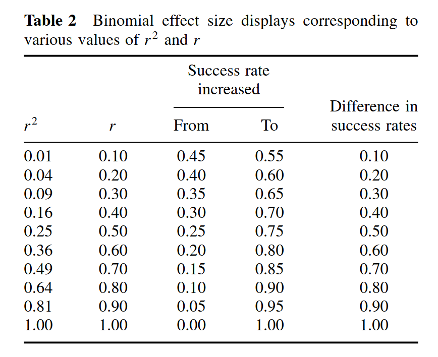
In this scenario, then, if you imagine a drug with an effect size of 0.20 d, or about 0.10 r. This would be a drug that has no immediately obvious effect, and would be somewhat difficult to notice without a large formal statistical study or prolonged professional experience (examples of sizes like this would be correlation between intelligence and crime, or intelligence and height). However, if we think about value as a treatment, it corresponds to increasing your chance of successful treatment from 50% to 55%. In other words, before you odds were 1-to-1 (50-50), but now your odds are 1.22 (55-to-45), that is, an increase of 22%. This may mean a lot to you if you are fighting a deadly disease or trying to hire a new, expensive employee. A correlation often designated as small, r = .30, “only explaining 9-10% of the variance”, then, would actually be a drastic improvement in your chances. From 50% to 65%. If you had a trick in the casino with this effectiveness, you would be a millionaire in a few hours work (assuming they don’t throw you out!).
In practice, you are not likely to have a scenario like this one with perfectly balanced outcomes, but it provides an intuitive way to see why values that sound small may not be so insignificant in real life. It depends on the situation. For good measure, there’s a variety of other criticism of the BESD, which you can read about here.