Most researchers don’t seem to think carefully about what they put in their regression models as statistical controls. By controlling for a variable, you attempt to hold that variable at a constant value while letting another variable vary to see what effect that has. If you include multiple controls, these are all kept constant insofar as possible with the given dataset. The usual interpretation applied to the model results usually assume a simple causal model namely that the dependent variable is caused by everything else directly, and these other variables aren’t caused by the dependent variable, and neither do they cause each other. If some of the predictors have causal relationships among each other, then the ultimate variables will have their effect size reduced to whichever effects that aren’t mediated by the other variables. For instance, if you predict wealth of a person as a function of their income and sex, you might find that men aren’t wealthier than women (controlling for income). In other words, men are wealthier but not if you look at men and women with the same income, or alternatively, that income differences explain all of the sex difference in wealth (I don’t know whether this is true, it’s an example.).
In many cases, researchers add as controls to their regression models just about every other variable they have, resulting in a so-called kitchen sink approach. They then interpret the discovered coefficients as the causal effects in some important sense. We saw an example of this yesterday with the German migrant crime data. Areas with more migrants aren’t more criminal than average (controlling for the unemployment rate, the German crime rate, the male %, and the mean age). This controls too much for the interpretation of the results to tell us about relevant causality (obviously, the migrants in low unemployment rate areas with low-crime Germans aren’t regular migrants, it’s improper to control for these factors). This kind of controlling for problematic variables error is sometimes called the Mount Everest regression fallacy (a few others have named other Everest fallacies unrelated to this). Mount Everest is not cold (controlling for altitude). This idea has been mentioned a few times (seems to be from Garett Jones), but no one seems to have empirically shown that it is true. So let’s try!
The data:
- There is a dataset of 10k towns with at least 10k population size here. It is based on Wikipedia and includes somewhat dirty climate data, but not altitude.
- I downloaded elevation (altitude) and annual temperature worldwide data from here. Then I looked up the location of each town + Mount Everest. This is not entirely precise because these are based on a grid of the Earth of 1 km² size. Mount Everest has an altitude of 8424 m here instead of the peak of 8848.
First, the correlations among the variables:
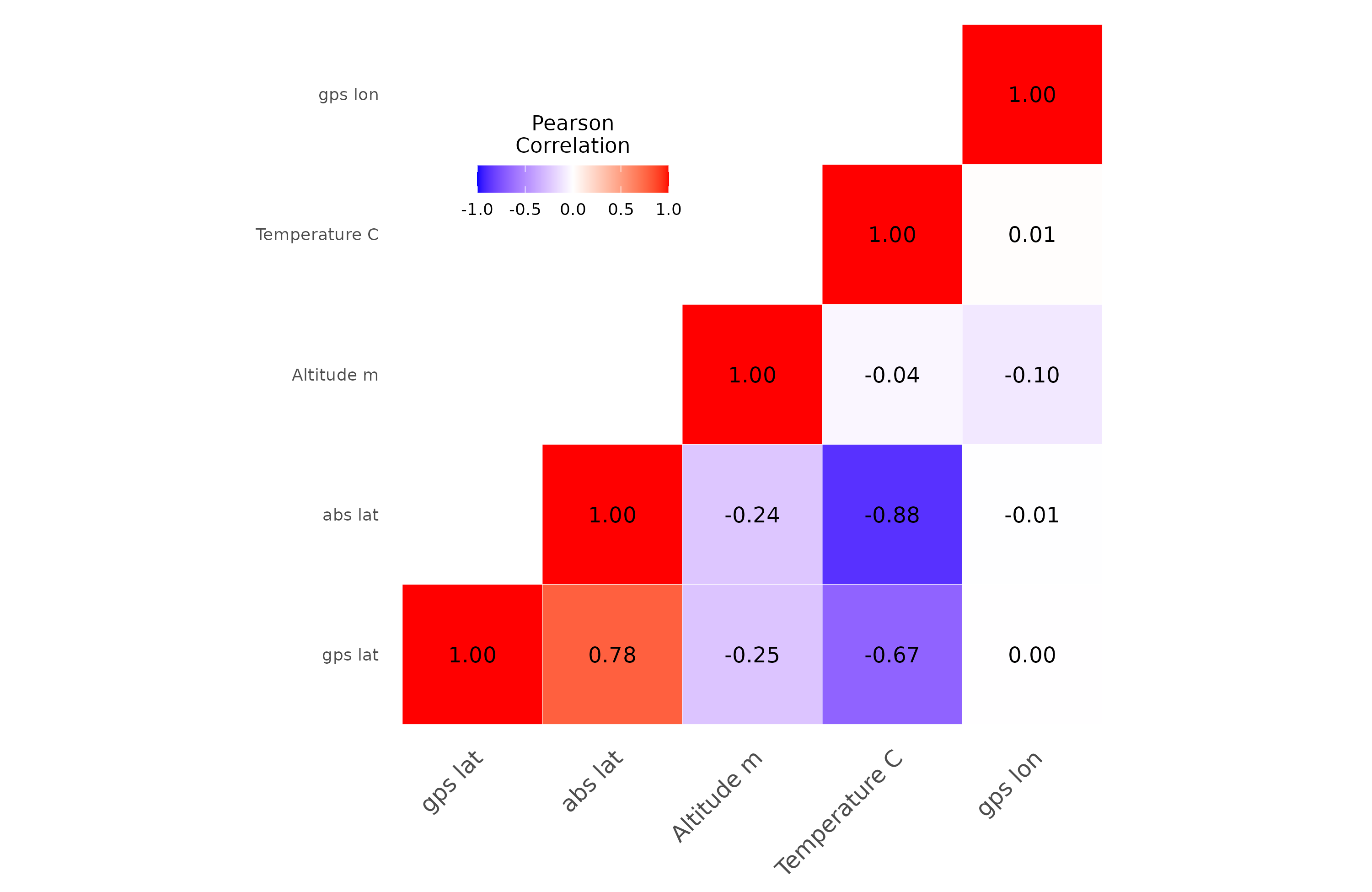
Mainly, temperature is predicted by latitude, not actually altitude. This is because the towns in mountains tend to be at warmer places (r = -0.24 with abs. latitude), presumably related to where humans choose to settle.
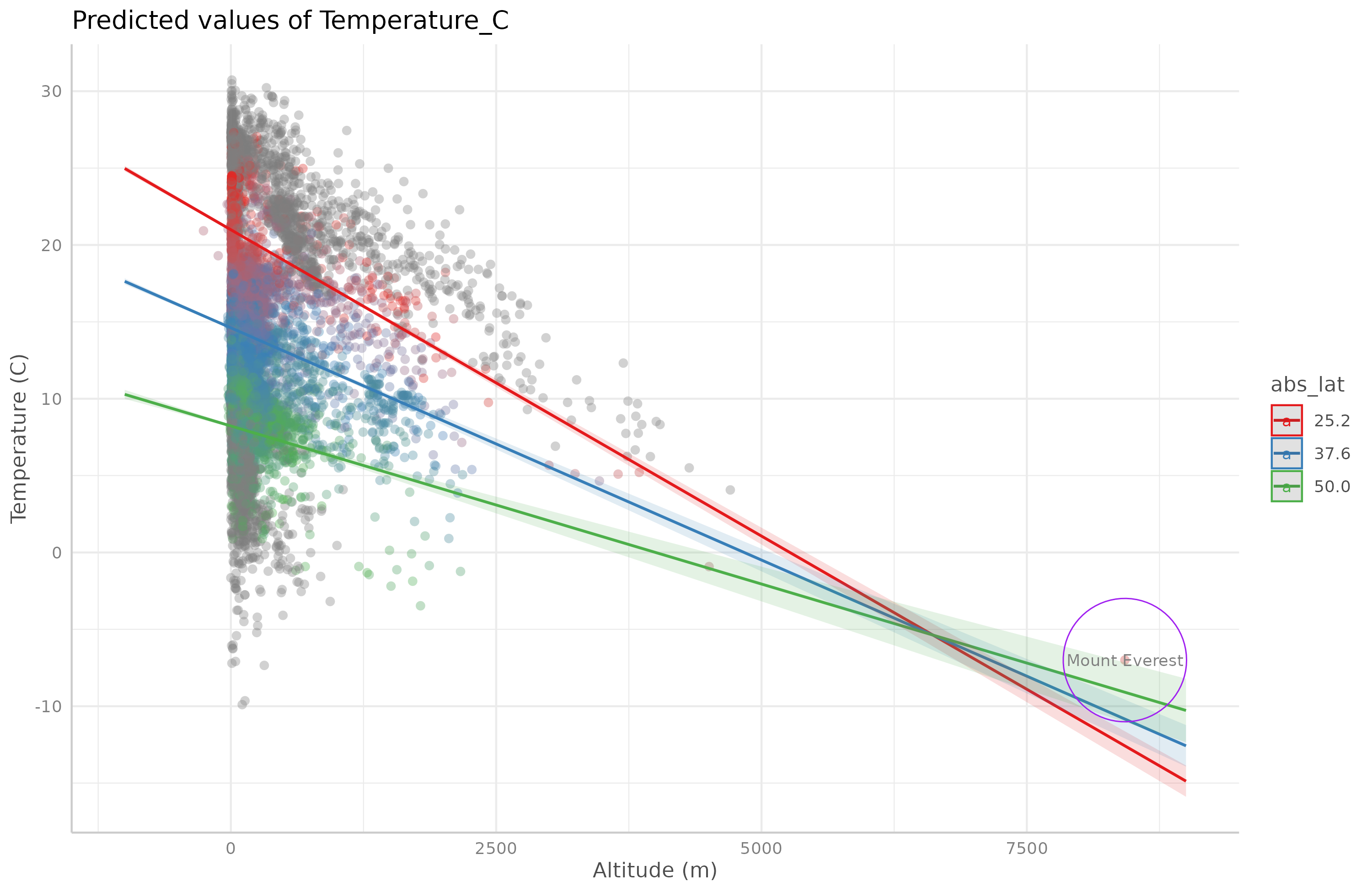
The pairwise relationships look like this:
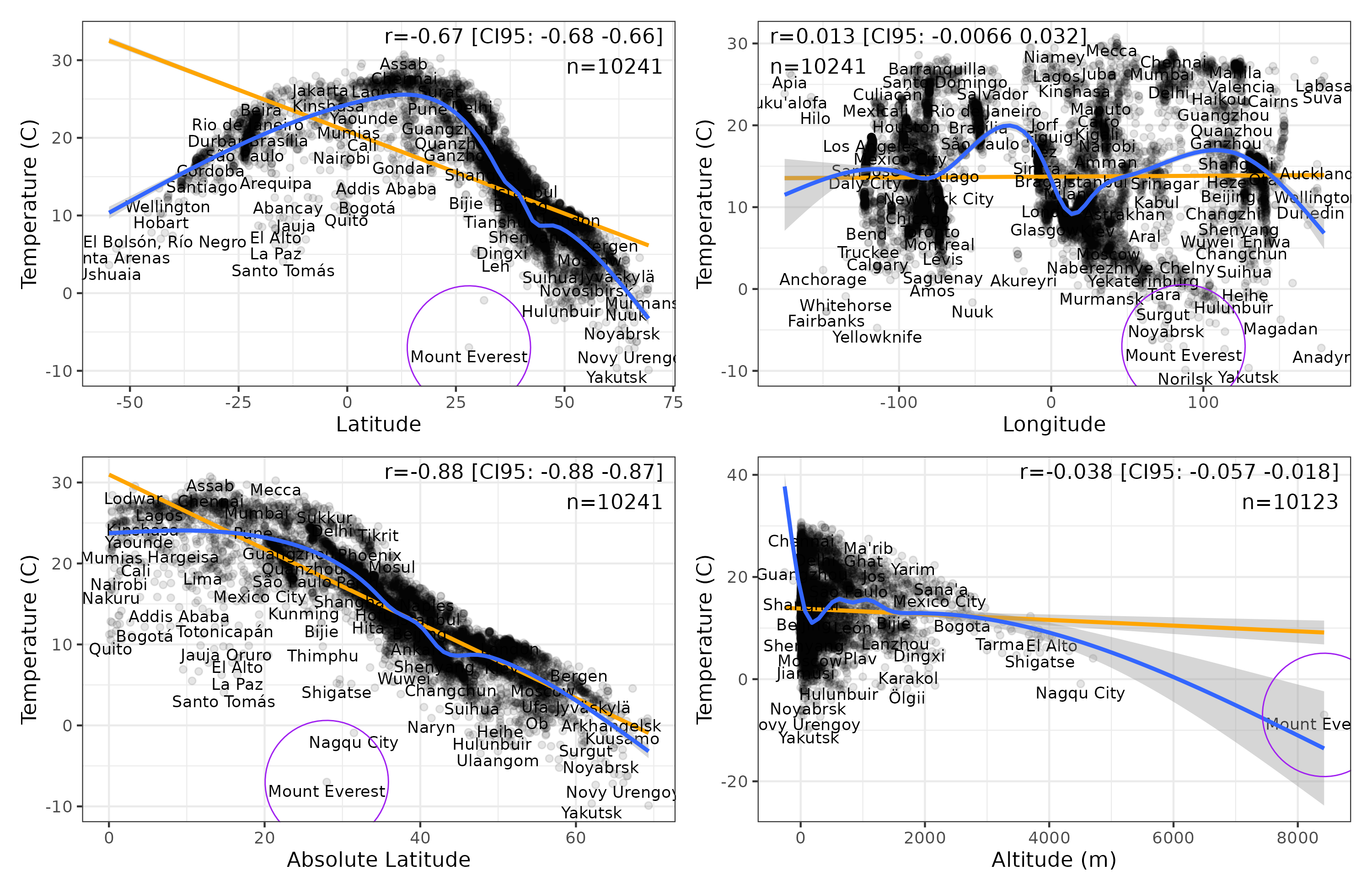
Mount Everest is a negative outlier for each of the simple relationships. Let’s try their combination:
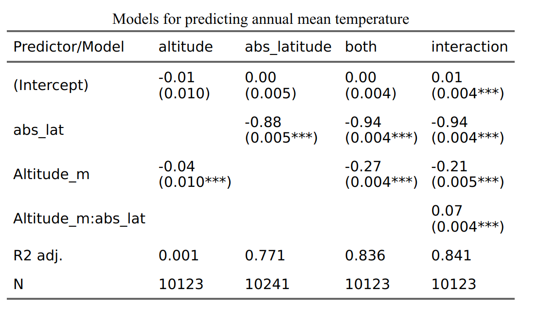
Altitude by itself explains just about nothing (r = -0.04), absolute latitude explains quite a lot (-0.88, 77% variance), their combination even more so (83.6% variance), and the interaction adds a bit more (84.1%). So, is Mount Everest actually cold (controlling for latitude and altitude)?
No, it turns out that Mount Everest is actually warm (controlling for altitude and latitude and their interaction). It is a positive outlier, so it is a few degrees warmer than expected!