Some time ago a new paper came out from the 23andme people reporting admixture among US ethnoracial groups (Bryc et al, 2014). Per our still on-going admixture project (current draft here), one could see if admixture predicts academic achievement (or IQ, if such were available). We (that is, John did) put together achievement data (reading and math scores) from the NAEP and the admixture data here.
Descriptive stats
Admixture studies do not work well if there is no or little variation within groups. So let’s first examine them. For blacks:
                      vars  n mean   sd median trimmed  mad  min  max range  skew kurtosis   se
BlackAfricanAncestry     1 31 0.74 0.04   0.74    0.74 0.03 0.64 0.83  0.19 -0.03    -0.38 0.01
BlackEuropeanAncestry    1 31 0.23 0.04   0.24    0.23 0.03 0.15 0.34  0.19  0.09    -0.30 0.01
So we see that there is little American admixture in Blacks because the African and European add up to close to 100 (23+74=97). In fact, the correlation between African and European ancestry in Blacks is -.99. This also means that multiple correlation is useless because of collinearity.
White admixture data is also not very useful. It is almost exclusively European:
                      vars  n mean sd median trimmed mad  min max range  skew kurtosis se
WhiteEuropeanAncestry    1 51 0.99  0   0.99    0.99   0 0.98   1  0.02 -0.95     0.74  0
What about Hispanics (some sources call them Latinos)?
                       vars  n mean   sd median trimmed  mad  min  max range skew kurtosis   se
LatinoEuropeanAncestry    1 34 0.73 0.07   0.72    0.73 0.05 0.57 0.90  0.33 0.34     0.22 0.01
LatinoAfricanAncestry     1 34 0.09 0.05   0.08    0.08 0.06 0.01 0.22  0.21 0.51    -0.69 0.01
LatinoAmericanAncestry    1 34 0.10 0.05   0.09    0.10 0.03 0.04 0.21  0.17 0.80    -0.47 0.01
Hispanics are fairly admixed. Overall, they are mostly European, but the range of African and American ancestry is quite high. Furthermore, due to the three way variation, multiple regression should work. The ancestry intercorrelations are: -.42 (Afro x Amer) -.21 (Afro x Euro) -.50 (Amer x Euro). There must also be another source because 73+9+10 is only 92%. Where’s the last 8% admixture from?
Admixture x academic achievement correlations: Blacks
| row.names | BlackAfricanAncestry | BlackAmericanAncestry | BlackEuropeanAncestry | |
|---|---|---|---|---|
| 1 | Math2013B | -0.32 | 0.09 | 0.29 |
| 2 | Math2011B | -0.27 | 0.21 | 0.25 |
| 3 | Math2009B | -0.30 | 0.09 | 0.28 |
| 4 | Math2007B | -0.12 | 0.27 | 0.08 |
| 5 | Math2005B | -0.28 | 0.26 | 0.23 |
| 6 | Math2003B | -0.30 | 0.15 | 0.26 |
| 7 | Math2000B | -0.36 | -0.08 | 0.34 |
| 8 | Read2013B | -0.25 | 0.14 | 0.22 |
| 9 | Read2011B | -0.33 | 0.22 | 0.30 |
| 10 | Read2009B | -0.40 | -0.03 | 0.41 |
| 11 | Read2007B | -0.26 | 0.14 | 0.24 |
| 12 | Read2005B | -0.43 | 0.33 | 0.39 |
| 13 | Read2003B | -0.42 | 0.09 | 0.38 |
| 14 | Read2002B | -0.30 | -0.10 | 0.27 |
Summarizing these results:
     vars  n  mean   sd median trimmed  mad   min   max range  skew kurtosis   se
Afro    1 14 -0.31 0.08  -0.30   -0.32 0.05 -0.43 -0.12  0.31  0.48     0.10 0.02
Amer    1 14  0.13 0.13   0.14    0.13 0.11 -0.10  0.33  0.43 -0.32    -1.07 0.03
Euro    1 14  0.28 0.08   0.28    0.29 0.06  0.08  0.41  0.33 -0.49     0.11 0.02
So we see the expected directions and order, for Blacks (who are mostly African), American admixture is positive and European is more positive. There is quite a bit of variation over the years. It is possible that this reflects mostly ‘noise’ as in, e.g. changes in educational policies in the states, or just sampling error. It is also possible that the changes are due to admixture changes within states over time.
Admixture x academic achievement correlations: Hispanics
| row.names | LatinoAfricanAncestry | LatinoAmericanAncestry | LatinoEuropeanAncestry | |
|---|---|---|---|---|
| 1 | Math13H | 0.20 | -0.13 | -0.10 |
| 2 | Math11H | 0.27 | 0.02 | -0.02 |
| 3 | Math09H | 0.29 | -0.32 | 0.04 |
| 4 | Math07H | 0.36 | -0.14 | -0.01 |
| 5 | Math05H | 0.38 | -0.08 | 0.00 |
| 6 | Math03H | 0.37 | -0.23 | -0.08 |
| 7 | Math00H | 0.30 | -0.09 | -0.05 |
| 8 | Read2013H | 0.18 | -0.44 | 0.33 |
| 9 | Read2011H | 0.21 | -0.26 | 0.33 |
| 10 | Read2009H | 0.19 | -0.44 | 0.33 |
| 11 | Read2007H | 0.13 | -0.32 | 0.23 |
| 12 | Read2005H | 0.38 | -0.30 | 0.23 |
| 13 | Read2003H | 0.32 | -0.34 | 0.18 |
| 14 | Read2002H | 0.24 | -0.23 | 0.08 |
And summarizing:
     vars  n  mean   sd median trimmed  mad   min  max range  skew kurtosis   se
Afro    1 14  0.27 0.08   0.28    0.28 0.12  0.13 0.38  0.25 -0.10    -1.49 0.02
Amer    1 14 -0.24 0.14  -0.24   -0.24 0.15 -0.44 0.02  0.46  0.17    -1.13 0.04
Euro    1 14  0.11 0.16   0.06    0.11 0.19 -0.10 0.33  0.43  0.23    -1.68 0.04
We do not see the expected results per genetic model. Among Hispanics who are 73% European, African admixture has a positive relationship to academic achievement. American admixture is negatively correlated and European positively, but weaker than African. The only thing that’s in line with the genetic model is that European is positive. On the other hand, results are not in line with a null model either, because then we were expecting results to fluctuate around 0.
Note that the European admixture numbers are only positive for the reading tests. The reading tests are presumably those mostly affected by language bias (many Hispanics speak Spanish as a first language). If anything, the math results are worse for the genetic model.
General achievement factors
We can eliminate some of the noise in the data by extracting a general achievement factor for each group. I do this by first removing the cases with no data at all, and then imputing the rest.
Then we get the correlation like before. This should be fairly close to the means above:
 LatinoAfricanAncestry LatinoAmericanAncestry LatinoEuropeanAncestry
                  0.28                  -0.36                   0.22
The European result is stronger with the general factor from the imputed dataset, but the order is the same.
We can do the same for the Black data to see if the imputation+factor analysis screws up the results:
 BlackAfricanAncestry BlackAmericanAncestry BlackEuropeanAncestry
                -0.35                  0.20                  0.31
These results are similar to before (-.31, .13, .28) with the American result somewhat stronger.
Plotting
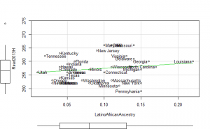
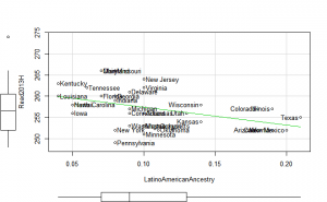
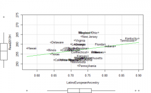
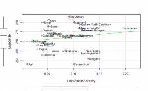
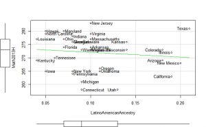
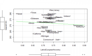
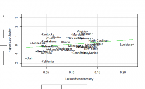
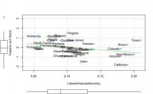
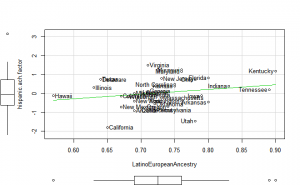
Perhaps if we plot the results, we can figure out what is going on. We can plot either the general achievement factor, or specific results. Let’s do both:
Reading2013 plots
Math2013 plots
General factor plots
These did not help me understand it. Maybe they make more sense to someone who understands US demographics and history better.
Multiple regression
As mentioned above, the Black data should be mostly useless for multiple regression due to high collinearity. But the hispanic should be better. I ran models using two of the three ancestry estimates at a time since one cannot use all three (I think).
Generally, the independents did not reach significance. Using the general achievement factor as the dependent, the standardized betas are:
LatinoAfricanAncestry LatinoAmericanAncestry
             0.1526765             -0.2910413
LatinoAfricanAncestry LatinoEuropeanAncestry
             0.3363636              0.2931108
LatinoAmericanAncestry LatinoEuropeanAncestry
           -0.32474678             0.06224425
The first is relative to European, second to American, and third African. The results are not even consistent with each other. In the first, African>European. In the third, European>African. All results show that Others>American tho.
The remainder
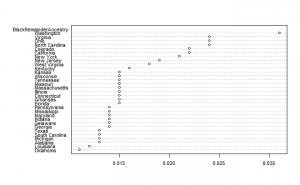
There is something odd about the data, it doesn’t sum to 1. I calculated the sum of the ancestry estimates, and then subtracted that from 1. Here’s the results:
To these we can add simple descriptive stats:
                        vars  n mean   sd median trimmed  mad  min  max range skew kurtosis   se
BlackRemainderAncestry     1 31 0.02 0.00   0.02    0.02 0.00 0.01 0.03  0.02 1.35     1.18 0.00
LatinoRemainderAncestry    1 34 0.08 0.05   0.07    0.07 0.03 0.02 0.34  0.32 3.13    12.78 0.01
So we see that there is a sizable other proportion of Hispanics and a small one for Blacks. Presumably, the large outlier of Hawaii is Asian admixture from Japanese, Chinese, Filipino and Native Hawaiian clusters. At least, these are the largest groups according to Wikipedia. For Blacks, the ancestry is presumably Asian admixture as well.
Do these remainders correlate with academic achievement? For Blacks, r = .39 (p = .03), and for Hispanics r = -.24 (p = .18). So the direction is as expected for Blacks and stronger, but for Hispanics, it is in the right direction but weaker.
Partial correlations
What about partialing out the remainders?
LatinoAfricanAncestry LatinoAmericanAncestry LatinoEuropeanAncestry
            0.21881404            -0.33114612             0.09329413
BlackAfricanAncestry BlackAmericanAncestry BlackEuropeanAncestry
           -0.2256171             0.1189219             0.2185139
Not much has changed. European correlation has become weaker for Hispanics. For Blacks, results are similar to before.
Proposed explanations?
The African results are in line with genetic models. The Hispanic is not, but it isn’t in line with the null-model either. Perhaps it has something to do with generational effects. Perhaps if one could find % of first generation Hispanics by state and add those to the regression model / control for that using partial correlations.
Other ideas? Before calculating the results, John wrote:
Language, generation, and genetic assimilation are all confounded, so I thought it best to not look at them.
He may be right.
R code
data = read.csv("BryceAdmixNAEP.tsv", sep="\t",row.names=1)
library(car) # for vif
library(psych) # for describe
library(VIM) # for imputation
library(QuantPsyc) #for lm.beta
library(devtools) #for source_url
#load mega functions
source_url("https://osf.io/project/zdcbq/osfstorage/files/mega_functions.R/?action=download")

#descriptive stats
#blacks
rbind(describe(data["BlackAfricanAncestry"]),
describe(data["BlackEuropeanAncestry"]))
#whites
describe(data["WhiteEuropeanAncestry"])
#hispanics
rbind(describe(data["LatinoEuropeanAncestry"]),
      describe(data["LatinoAfricanAncestry"]),
      describe(data["LatinoAmericanAncestry"]))

##Regressions
#Blacks
black.model = "Math2013B ~ BlackAfricanAncestry+BlackAmericanAncestry"
black.model = "Read2013B ~ BlackAfricanAncestry+BlackAmericanAncestry"
black.model = "Math2013B ~ BlackAfricanAncestry+BlackEuropeanAncestry"
black.model = "Read2013B ~ BlackAfricanAncestry+BlackEuropeanAncestry"
black.fit = lm(black.model, data)
summary(black.fit)

#Hispanics
hispanic.model = "Math2013H ~ LatinoAfricanAncestry+LatinoAmericanAncestry"
hispanic.model = "Read2013H ~ LatinoAfricanAncestry+LatinoAmericanAncestry"
hispanic.model = "Math2013H ~ LatinoAfricanAncestry+LatinoEuropeanAncestry"
hispanic.model = "Read2013H ~ LatinoAfricanAncestry+LatinoEuropeanAncestry"
hispanic.model = "hispanic.ach.factor ~ LatinoAfricanAncestry+LatinoAmericanAncestry"
hispanic.model = "hispanic.ach.factor ~ LatinoAfricanAncestry+LatinoEuropeanAncestry"
hispanic.model = "hispanic.ach.factor ~ LatinoAmericanAncestry+LatinoEuropeanAncestry"
hispanic.model = "hispanic.ach.factor ~ LatinoAfricanAncestry+LatinoAmericanAncestry+LatinoEuropeanAncestry"
hispanic.fit = lm(hispanic.model, data)
summary(hispanic.fit)
lm.beta(hispanic.fit)

##Correlations
cors = round(rcorr(as.matrix(data))$r,2) #all correlations, round to 2 decimals

#blacks
admixture.cors.black = cors[10:23,1:3] #Black admixture x Achv.
hist(unlist(admixture.cors.black[,1])) #hist for afri x achv
hist(unlist(admixture.cors.black[,2])) #amer x achv
hist(unlist(admixture.cors.black[,3])) #euro x achv
desc = rbind(Afro=describe(unlist(admixture.cors.black[,1])), #descp. stats afri x achv
             Amer=describe(unlist(admixture.cors.black[,2])), #amer x achv
             Euro=describe(unlist(admixture.cors.black[,3]))) #euro x achv

#whites
admixture.cors.white = cors[24:25,4:6] #White admixture x Achv.

#hispanics
admixture.cors.hispanic = cors[26:39,7:9] #White admixture x Achv.
desc = rbind(Afro=describe(unlist(admixture.cors.hispanic[,1])), #descp. stats afri x achv
             Amer=describe(unlist(admixture.cors.hispanic[,2])), #amer x achv
             Euro=describe(unlist(admixture.cors.hispanic[,3]))) #euro x achv

##Examine hispanics by scatterplots
#Reading
scatterplot(Read2013H ~ LatinoAfricanAncestry, data,
            smoother=FALSE, id.n=nrow(data))
scatterplot(Read2013H ~ LatinoEuropeanAncestry, data,
            smoother=FALSE, id.n=nrow(data))
scatterplot(Read2013H ~ LatinoAmericanAncestry, data,
            smoother=FALSE, id.n=nrow(data))
#Math
scatterplot(Math2013H ~ LatinoAfricanAncestry, data,
            smoother=FALSE, id.n=nrow(data))
scatterplot(Math2013H ~ LatinoEuropeanAncestry, data,
            smoother=FALSE,id.n=nrow(data))
scatterplot(Math2013H ~ LatinoAmericanAncestry, data,
            smoother=FALSE,id.n=nrow(data))
#General factor
scatterplot(hispanic.ach.factor ~ LatinoAfricanAncestry, data,
            smoother=FALSE, id.n=nrow(data))
scatterplot(hispanic.ach.factor ~ LatinoEuropeanAncestry, data,
            smoother=FALSE,id.n=nrow(data))
scatterplot(hispanic.ach.factor ~ LatinoAmericanAncestry, data,
            smoother=FALSE,id.n=nrow(data))

##Imputed and aggregated data
#Hispanics
hispanic.ach.data = data[26:39] #subset hispanic ach data
hispanic.ach.data = hispanic.ach.data[miss.case(hispanic.ach.data)<ncol(hispanic.ach.data),] #remove empty cases
miss.table(hispanic.ach.data) #examine missing data
hispanic.ach.data = irmi(hispanic.ach.data, noise.factor = 0) #impute the rest
#factor analysis
fact.hispanic = fa(hispanic.ach.data) #get common ach factor
fact.scores = fact.hispanic$scores; colnames(fact.scores) = "hispanic.ach.factor"
data = merge.datasets(data,fact.scores,1) #merge it back into data
cors[7:9,"hispanic.ach.factor"] #results for general factor

#Blacks
black.ach.data = data[10:23] #subset black ach data
black.ach.data = black.ach.data[miss.case(black.ach.data)<ncol(black.ach.data),] #remove empty cases
black.ach.data = irmi(black.ach.data, noise.factor = 0) #impute the rest
#factor analysis
fact.black = fa(black.ach.data) #get common ach factor
fact.scores = fact.black$scores; colnames(fact.scores) = "black.ach.factor"
data = merge.datasets(data,fact.scores,1) #merge it back into data
cors[1:3,"black.ach.factor"] #results for general factor

##Admixture totals
#Hispanic
Hispanic.admixture = subset(data, select=c("LatinoAfricanAncestry","LatinoAmericanAncestry","LatinoEuropeanAncestry"))
Hispanic.admixture = Hispanic.admixture[miss.case(Hispanic.admixture)==0,] #complete cases
Hispanic.admixture.sum = data.frame(apply(Hispanic.admixture, 1, sum))
colnames(Hispanic.admixture.sum)="Hispanic.admixture.sum" #fix name
describe(Hispanic.admixture.sum) #stats

#add data back to dataframe
LatinoRemainderAncestry = 1-Hispanic.admixture.sum #get remainder
colnames(LatinoRemainderAncestry) = "LatinoRemainderAncestry" #rename
data = merge.datasets(LatinoRemainderAncestry,data,2) #merge back

#plot it
LatinoRemainderAncestry = LatinoRemainderAncestry[order(LatinoRemainderAncestry,decreasing=FALSE),,drop=FALSE] #reorder
dotchart(as.matrix(LatinoRemainderAncestry),cex=.7) #plot, with smaller text

#Black
Black.admixture = subset(data, select=c("BlackAfricanAncestry","BlackAmericanAncestry","BlackEuropeanAncestry"))
Black.admixture = Black.admixture[miss.case(Black.admixture)==0,] #complete cases
Black.admixture.sum = data.frame(apply(Black.admixture, 1, sum))
colnames(Black.admixture.sum)="Black.admixture.sum" #fix name
describe(Black.admixture.sum) #stats

#add data back to dataframe
BlackRemainderAncestry = 1-Black.admixture.sum #get remainder
colnames(BlackRemainderAncestry) = "BlackRemainderAncestry" #rename
data = merge.datasets(BlackRemainderAncestry,data,2) #merge back

#plot it
BlackRemainderAncestry = BlackRemainderAncestry[order(BlackRemainderAncestry,decreasing=FALSE),,drop=FALSE] #reorder
dotchart(as.matrix(BlackRemainderAncestry),cex=.7) #plot, with smaller text

#simple stats for both
rbind(describe(BlackRemainderAncestry),describe(LatinoRemainderAncestry))

#make subset with remainder data and achievement
remainders = subset(data, select=c("black.ach.factor","BlackRemainderAncestry",
                                   "hispanic.ach.factor","LatinoRemainderAncestry"))
View(rcorr(as.matrix(remainders))$r) #correlations?

#Partial correlations
partial.r(data, c(7:9,40), c(43))[4,] #partial out remainder for Hispanics
partial.r(data, c(1:3,41), c(42))[4,] #partial out remainder for Blacks
References
Bryc, K., Durand, E. Y., Macpherson, J. M., Reich, D., & Mountain, J. L. (2014). The Genetic Ancestry of African Americans, Latinos, and European Americans across the United States. The American Journal of Human Genetics.
