Blog

Attacking a study for using a non-representative, typically online convenience sample is common practice. However, for most studies, this is wrong-headed and here I want to argue why that is so. AellaGirl recently caused a lot of these reactions because she analyzed huge convenience samples of her own followers on various platforms. Back in December of 2022, she wrote a post defending this practice You don’t need a perfectly random sample for useful data, jfc. Of course, since most social science is done using such non-representative datasets, the criticism would be hypocritical if it came from psychologists. But we don’t need to rely on tu quoque retorts. We just need to think about how sampling bias affects results in studies.

Let’s begin with the most obvious case where you are trying to estimate a population mean. Suppose you want to know who is going to be the next president. Ignoring the details of weird election systems, let’s pretend this comes down to a run-off election with 2 choices as done in France. All you need to do here is figure out whether the voters like candidate A or B more. So really, you just need to estimate the proportion of voters who prefer A, as B is the complement. If you tried doing this using convenience samples, you would probably not make very good predictions. The reason for this is that it’s quite easy to end up with a sample that isn’t representative for preferring one candidate over another because candidate preference is usually correlated with age, sex, location, educational level and so on. Convenience samples, such as university students, are usually younger, more female, higher educated (eventually) and concentrated in urban areas. Pollsters of course know about this so they have a big statistical toolkit for trying to debias the results, usually with good results.

But most studies are not like the above. They aren’t trying to estimate a simple mean (a univariate statistic). Rather, they are trying to estimate the relationship between various variables, which would be a bivariate or multivariate statistic. These are much more robust to sampling bias than univariate statistics. You can think of the possible reasons why. For the value to differ between two samples or subgroups, there must be:

1. An interaction of the actual relationship and the sample/group, or
2. Variance differences which affect some statistics but not others, or
3. Some kind of sneaky selection problem that results in collider bias

Each potential problem can be tackled in part. The 1st possibility is popular but mostly false. The 2nd possibility is ubiquitous but relatively easy to adjust for, and does not always give a bias (it depends on whether it is in the dependent or independent variable and whether you use standardized or raw slopes). And when it gives a bias, it is not usually extreme, and cannot result in opposite directions of estimates (variance bias might change your correlation from .50 to .35). The 3rd problem is the most tricky because it can in rare cases reverse the direction of the result. Julia Rohrer has an example on her blog.

Fortunately, it is empirically possible to check how often true differences in effects (relationships between variables) exist ‘in nature’. Here are some studies I found:

Surveys of various types

Survey experiments generalize very well across most groups and samples in a systemic study of 27 experiments.

• Coppock, A., Leeper, T. J., & Mullinix, K. J. (2018). Generalizability of heterogeneous treatment effect estimates across samples. Proceedings of the National Academy of Sciences, 115(49), 12441-12446.

The extent to which survey experiments conducted with nonrepresentative convenience samples are generalizable to target populations depends critically on the degree of treatment effect heterogeneity. Recent inquiries have found a strong correspondence between sample average treatment effects estimated in nationally representative experiments and in replication studies conducted with convenience samples. We consider here two possible explanations: low levels of effect heterogeneity or high levels of effect heterogeneity that are unrelated to selection into the convenience sample. We analyze subgroup conditional average treatment effects using 27 original–replication study pairs (encompassing 101,745 individual survey responses) to assess the extent to which subgroup effect estimates generalize. While there are exceptions, the overwhelming pattern that emerges is one of treatment effect homogeneity, providing a partial explanation for strong correspondence across both unconditional and conditional average treatment effect estimates.

And here’s a prior similar study:

• Mullinix, K. J., Leeper, T. J., Druckman, J. N., & Freese, J. (2015). The generalizability of survey experiments. Journal of Experimental Political Science, 2(2), 109-138.

Survey experiments have become a central methodology across the social sciences. Researchers can combine experiments’ causal power with the generalizability of population-based samples. Yet, due to the expense of population-based samples, much research relies on convenience samples (e.g. students, online opt-in samples). The emergence of affordable, but non-representative online samples has reinvigorated debates about the external validity of experiments. We conduct two studies of how experimental treatment effects obtained from convenience samples compare to effects produced by population samples. In Study 1, we compare effect estimates from four different types of convenience samples and a population-based sample. In Study 2, we analyze treatment effects obtained from 20 experiments implemented on a population-based sample and Amazon’s Mechanical Turk (MTurk). The results reveal considerable similarity between many treatment effects obtained from convenience and nationally representative population-based samples. While the results thus bolster confidence in the utility of convenience samples, we conclude with guidance for the use of a multitude of samples for advancing scientific knowledge.

Validity generalization

There is a subfield of psychology that studies work, usually called industrial-organization (I/O) psychology. In this field researchers produced a lot of quite small studies that looked at whether intelligence predicts job performance across job types. They concluded that the effects were totally inconsistent, so that a test that might work for job X, didn’t work for job X in another company, or very similar job Y in the same company. This is the same as claiming that there are massive interactions everywhere. The error here was mainly one of statistics. When you have two small studies, one which finds p < .05, and one which doesn’t, this pattern of p values does not really give you much evidence of a difference in effect sizes. Rather, it is possible the true effect size is the same across these studies and settings and the differences are due to random noise (sampling error). Differences can also be due to ‘range restriction’, i.e., when you have a sample that has less variance for some personality trait (e.g. intelligence) because it has already been selected (e.g. comparing incumbent workers vs. applicants). Some smart people in this field figured out how to do real tests for such interactions and methods for adjusting for known/estimated biases of the data. A summary from a 2014 introduction book:

In personnel selection, it had long been believed that validity was specific to situations; that is, it was believed that the validity of the same test for what appeared to be the same job varied from employer to employer, region to region, across periods, and so forth. In fact, it was believed that the same test could have high validity (i.e., a high correlation with job performance) in one location or organization and be completely invalid (i.e., have zero validity) in another. This belief was based on the observation that observed validity coefficients for similar tests and jobs (and even for the same test and job over time) varied substantially across different studies. In some studies, there was a statistically significant relationship, and in others, there was no significant relationship—which was falsely taken to indicate there was no relationship at all. This puzzling variability of findings was explained by postulating that jobs that appeared to be the same actually differed in important ways in what was required to perform them. This belief led to a requirement for local or situational validity studies. It was held that validity had to be estimated separately for each situation by a study conducted in that setting; that is, validity findings could not be generalized across settings, situations, employers, and the like (Schmidt & Hunter, 1981). In the late 1970s, meta-analysis of validity coefficients began to be conducted to test whether validity might not, in fact, be generalizable (Schmidt & Hunter, 1977; Schmidt, Hunter, Pearlman, & Shane, 1979), and, thus, these meta-analyses were called “validity generalization” studies. These studies indicated that all or most of the study-to-study variability in observed validities was due to artifacts of the kind discussed in this book and that the traditional belief in situational specificity of validity was therefore erroneous. Validity findings did generalize.

The math is complicated, but to get the basic idea consider a bunch of studies with small sample sizes trying to estimate the relationship between intelligence and job performance for firemen. It might look something like this:

So looking across the various studies, they do seem very inconsistent. Study 1 finds basically no effect, study 10 finds a large one. But if you eyeball the 20 confidence intervals you see that they almost entirely overlap a central value of .30ish. The weighted mean is .32 with a standard deviation of .10. If one assumes a true correlation of .32 that is constant across studies and the variation due only to sampling error, one finds that there isn’t much variation between studies left to explain. That’s what the various heterogeneity tests tell you. In this case, the leftover variance between studies is about 12% of the total variance, which is not beyond what is expected by chance.

In I/O psychology, they have run 100s of such meta-analyses and generally they find that sampling error and data biases explain most variation between studies which also means that there isn’t much true differences in the effects between studies.

Interactions do not generally replicate (OKCupid)

In 2018, Jonatan Pallesen did an empirical demonstration of this using the large OKCupid dataset based on a prior study by me (Rpubs are here and here). The idea:

Many social psychology studies are about interaction effects, and many of these have had unsuccessful replications. Interaction effects are found to be especially prone to fail replication in the replication project, and in this study.

In this document I explore whether interaction effects are less likely to replicate as a general rule, in a real, large data set. The data set is from the users’ answers to a large number of personal questions in the OKCupid data set.

We find that significant interaction effects explain very little of the variance, and that compared to significant main effects they are less significant, and are much less likely to replicate in a larger sample.

For the third variable we include either another ordinal variable, or gender. We find that interaction effects only replicate at 0.05 in ~9% of cases for ordinal variables, and ~22% for gender. Whereas main effects replicate in >95% of cases for either.

If we look at gender-specific effects (effects that are only significant for one gender), the replication mostly gives a non-gender-specific effect, and is very unlikely to find an effect only in that gender.

Method

I generate 1,000,000 random regressions using the OKCupid data. An example of a regression would be:

y = “Do you like to listen to audiobooks?” a = “How was your childhood?”
b = gender

y = a + b + a * b

I look at main effects(a, b) and interaction effects (a * b).

I do this in a sample with the answers of 500 people. Then I look at the same regression in a larger sample of 5,000 people, and see whether the results that are significant in the n = 500 sample, are also significant in the larger sample.

For instance, one result could be that people who like audiobooks tend to have had a good childhood. This type of main effect result typically is replicated in the n = 5,000 sample.

Or another result could be that there is a significant interaction between gender and childhood quality in predicting whether the person likes audiobooks. This type of effect is typically not replicated in the n = 5,000 sample.

Visually:

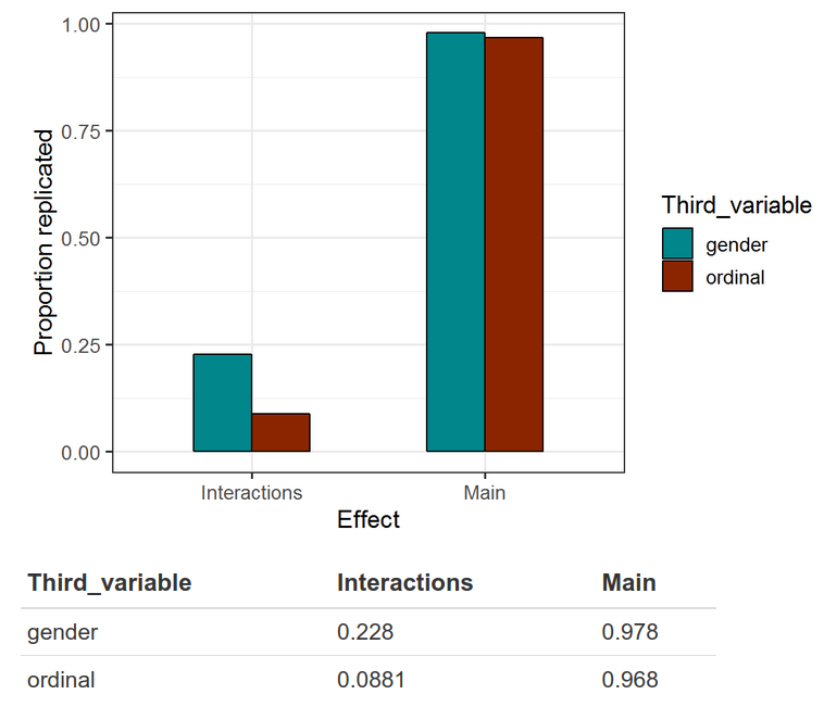
In other words, whenever some study claims an interaction effect based on p < .05 using a sample size of 500, this only replicates about 8% of the time (5% is expected by chance). When that claimed interaction value is sex, it replicates about 23% of the time (vs. 5% by chance). The main effects replicate more than 95% of the time. Now recall that most studies in social science do not have sample sizes of 500, but smaller, so their results would be even worse. The Rpubs goes into more detail, such as applying power analysis, p-curves and so on. But basically if you want to claim an interaction that doesn’t have an airtight expectation, you need to use something more better than p < .05 as your threshold, maybe p < .005 is a good start. The interaction effects that are found are usually also fairly trivial in size compared to the main effects. Importantly, real interactions very rarely produce opposite sign effects, or effects that only exist for one sex and not another. These make for interesting theories stories, but poor science.

Gene by environment (GxE) interactions

We’ve been over these quite a few times on the blog, so let’s keep it short here. There are two ways to study these. First, you can study individual genetic variants or polygenic scores, and interact these with some environmental variables (recall that these are also heritable to some extent, so this is not really pure GxE). Second, you can look at family data and see if the variance components for phenotypes differ by some third variable.

The candidate genetics era research has by now been more or less completely discredited. It was never plausible to begin with. This is also true for the GxE sub-type. In this line of research, researchers looked to predict behavior or something by whether specific genetic variants occurred with some environmental trigger or not. Typical of this era is the 5-HTTLPR variant. This was supposed to interact with bad environments to produce depression (or whatever). Scott Alexander has written the best write-up on this research. The TL;DR is that these are all false positives, nothing replicates in proper large planned studies. 10+ years of self-delusion. Dalliard hilariously commented on some philosophers who hadn’t gotten the memo in 2022:

On the causal interpretation of heritability from a structural causal modeling perspective by Lu & Bourrat. According to the authors, the “current consensus among philosophers of biology is that heritability analysis has minimal causal implications.” Except for rare dissenters like the great Neven Sesardic, philosophers seem to never have been able to move on from the arguments against heritability estimation that Richard Lewontin made in the 1970s. Fortunately, quantitative and behavioral geneticists have paid no attention to philosophers’ musings on the topic, and have instead soldiered on, collecting tons of new genetically informative data and developing numerous methods so as to analyze genetic causation. Lu & Bourrat’s critique of behavioral genetic decompositions of phenotypic variance is centered on gene-environment interactions and correlations. They write that “there is emerging evidence of substantial interaction in psychiatric disorders; therefore, deliberate testing of interaction hypotheses involving meta-analysis has been suggested (Moffitt et al., 2005).” That they cite a 17-year-old paper from the candidate gene era as “emerging evidence” in 2022 underlines the fact that the case for gene-environment interactions remains empirically very thin, despite its centrality to the worldview of the critics of behavioral genetics (see Border et al., 2019 regarding the fate of the research program by Moffitt et al.).

The newer version of this research is interacting polygenic scores with environmental variables in order to improve predictions. This has also been more or less a nothing-burger. E.g. Allegrini et al 2020:

Polygenic scores are increasingly powerful predictors of educational achievement. It is unclear, however, how sets of polygenic scores, which partly capture environmental effects, perform jointly with sets of environmental measures, which are themselves heritable, in prediction models of educational achievement. Here, for the first time, we systematically investigate gene-environment correlation (rGE) and interaction (GxE) in the joint analysis of multiple genome-wide polygenic scores (GPS) and multiple environmental measures as they predict tested educational achievement (EA). We predict EA in a representative sample of 7,026 16-year-olds, with 20 GPS for psychiatric, cognitive and anthropometric traits, and 13 environments (including life events, home environment, and SES) measured earlier in life. Environmental and GPS predictors were modelled, separately and jointly, in penalized regression models with out-of-sample comparisons of prediction accuracy, considering the implications that their interplay had on model performance. Jointly modelling multiple GPS and environmental factors significantly improved prediction of EA, with cognitive-related GPS adding unique independent information beyond SES, home environment and life events. We found evidence for rGE underlying variation in EA (rGE = .38; 95% CIs = .30, .45). We estimated that 40% (95% CIs = 31%, 50%) of the polygenic scores effects on EA were mediated by environmental effects, and in turn that 18% (95% CIs = 12%, 25%) of environmental effects were accounted for by the polygenic model, indicating genetic confounding. Lastly, we did not find evidence that GxE effects significantly contributed to multivariable prediction. Our multivariable polygenic and environmental prediction model suggests widespread rGE and unsystematic GxE contributions to EA in adolescence.

That is, despite a sample size of 7000+ people with 20 different polygenic scores and 13 different environment measures, they cannot find much of anything where modeling GxE adds anything beyond chance levels. There’s a 2023 replication as well (von Stumm et al 2023): “No consistent gene-environment interactions (GxE) were observed”.

The second approach of variance metrics doesn’t fare much better. It too has had great publicity. Most famously, Turkheimer’s 2003 research trying to show that heritability differs dramatically by social status (SES) level such that low SES lowers the importance of genetics. The 2015 meta-analysis of these studies found no overall such GxE worldwide, and only in their US-subset of studies did they find some evidence (exploratory subset analysis). It also showed that Turkheimer’s 2003 study was a massive outlier.

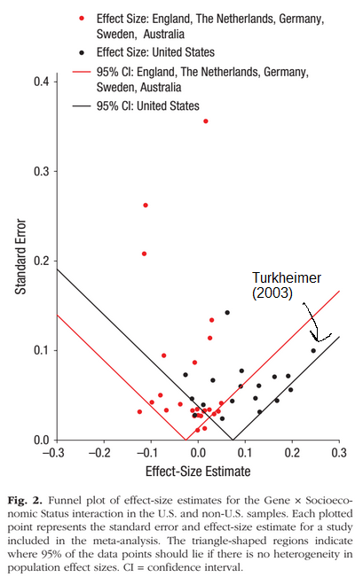
Their study also showed publication bias in the US context, and a much larger replication using register data from 50,000+ twins found no evidence even in the American context (Figlio et al 2017). There isn’t a single validated GxE except for heritability increasing with age while the shared environment decreases (the Wilson effect). This is not surprising. Kids are heavily influenced by their parents while living at home, but this is starkly reduced as they gain independence in adolescence and fades away in adulthood for the most part.

Implications for personalized medicine

The conclusions from this kind of reasoning are actually far-reaching for everyday life. Very commonly you will hear people arguing that something “works well for them”, but not for someone else. This is often claimed with medicine for common ailments. Someone might claim that treatment X “worked for them”, but “didn’t work for their friend”. Really, they are asserting an interaction effect of some sort where treatments can have dramatically different effects for otherwise similar people. This is nonsense. Such anecdotal data cannot show anything like that, it cannot even show main effects, which is why we demand randomized trials to begin with. As we saw in the OKCupid results, even using large samples of 500 people, it is difficult to detect real interaction effects between variables. It is comical to think one can find such effects based on casual observations. The correct approach when someone makes claims like these is to ignore them and look for some proper science. If some treatment worked well enough in a medical trial to get approved, it also works for you with 99%+ probability. You might not see an immediate effect when using it, but that is of course because the effects of most medicine are too small to see in casual observations. You don’t stop taking aspirin against heart attacks just because you can’t see a difference. You have to trust the science.

In fact, the enterprise of personalized medicine is largely undermined based on these considerations. There are in general no large interactions that one can find for a given patient with regards to what drugs work for them. The main exception to this is cancer therapy because the effectiveness of treatments depend on the mutations in the cancer which are unique, or at least come in several known clusters. If you have a run-of-the-mill ailment (e.g. cold, herpes, broken bone), you better stick with whatever works for everybody else as demonstrated in the relevant medical trials.