-
Lawson, D. J., Davies, N. M., Haworth, S., Ashraf, B., Howe, L., Crawford, A., … & Timpson, N. J. (2020). Is population structure in the genetic biobank era irrelevant, a challenge, or an opportunity?. Human genetics, 139(1), 23-41.
Replicable genetic association signals have consistently been found through genome-wide association studies in recent years. The recent dramatic expansion of study sizes improves power of estimation of effect sizes, genomic prediction, causal inference, and polygenic selection, but it simultaneously increases susceptibility of these methods to bias due to subtle population structure. Standard methods using genetic principal components to correct for structure might not always be appropriate and we use a simulation study to illustrate when correction might be ineffective for avoiding biases. New methods such as trans-ethnic modeling and chromosome painting allow for a richer understanding of the relationship between traits and population structure. We illustrate the arguments using real examples (stroke and educational attainment) and provide a more nuanced understanding of population structure, which is set to be revisited as a critical aspect of future analyses in genetic epidemiology. We also make simple recommendations for how problems can be avoided in the future. Our results have particular importance for the implementation of GWAS meta-analysis, for prediction of traits, and for causal inference.
This paper came out some time ago, and I tweeted it, but it’s worth compiling the good parts here as well for a more permanent record.
This paper finally provides a neat, visual introduction to what “controlling for population stratification” really means, and most importantly, why one cannot just blindly do it. As they explain:
Population structure is correlated with phenotypes
To understand why effect estimates may be biased, it is helpful to revisit ideas in population genetics. Populations do differ genetically by genetic drift and/or selection, and as a consequence these populations will also have different genetic phenotypes. For example, ancient populations had different “genetic heights” (Mathieson et al. 2015), with some potentially being taller than any modern population. Height, and other traits, appear to be “omnigenic” (Boyle et al. 2017); that is, there is no region of the genome not in linkage disequilibrium (LD) with SNPs causal for these traits. Since modern populations are a mixture of older populations, SNPs causal for the trait are themselves correlated with ancestry. It follows that the estimate of the effect of a SNP on a trait can be an underestimate when correcting for population structure.
The justification for PCA correction for population structure (Price et al. 2006) is to correct for non–causal linear associations between ancestry and phenotype (Fig. 1a). Causality is hard to define because we rarely measure the exact cause, but proxy it; here we are interested in proxies that are genetic and act through biological pathways. A non-causal association can be generated when population structure is associated with both allele frequency and the phenotype (Fig. 1a). For example, genetic drift simultaneously changes phenotype and SNP frequencies by chance. Weak genetic drift as experienced by larger populations over short timescales is additive, which corresponds to an additive effect on PCs (McVean 2009). Larger genetic drift, as produced by extreme bottlenecks or consanguinity, is not additive as the SNP frequency distribution becomes skewed and SNPs may become fixed or lost from a population. PCA correction and related methods are less useful when such drifted populations are included (Lawson et al. 2018).
Admixture can change SNP frequencies genome-wide, and small admixture variation is ubiquitous. Even large modern human populations not homogeneous—each individual has a slightly different ancestry proportion from earlier populations. The most ancient detectible human admixture event—Neanderthal introgression into Eurasians—has a mean of around 2% (Sankararaman et al. 2014), but varies substantially between populations and individuals (Wall et al. 2013). Many features of Neanderthal ancestry can be correctly understood using GWAS, which is associated causally with some phenotypes including increasing the risk of depression (Simonti et al. 2016), and non-causally with others, for example skin color (because Neanderthal genes entered the modern human gene pool outside of Africa).
I.e., authors introduce the idea that ancestry may be causally related to phenotypes, and give an example where non-Africans may suffer various issues due to Neanderthal admixture. Very PC.
Admixture has the potential to interact with family studies. Siblings have the same expected value of ancestry, with them both receiving a random realized amount. Realized, rather than expected, ancestry is a better predictor of phenotypes (Speed and Balding 2015). Such admixture variation can tag an environmental covariate, for example alcohol consumption influenced by ALDH2 (Price et al. 2002). It could also tag another phenotype that has a confounding relationship, for example, when mixed-race siblings vary in skin tone they may experience different societal pressures (Song 2010), which would be plausibly associated with educational attainment (Light and Strayer 2002) and other phenotypes. A causal analysis would include this pathway—i.e., in the examples, ALDH2 is causal for alcohol consumption and skin tone for education. However, in the second example the inference does not fit our definition of being biologically caused since it is mediated solely through modifiable societal norms.
That’s right: siblings are great in theory for admixture/ancestry analysis. Naturally, the idea is not new. It originates with none other than William Shockley who introduced it in an obscure science paper in 1966!
-
Shockley, W. (1966, January). Possible transfer of metallurgical and astronomical approaches to problem of environment versus ethnic heredity. In Science (Vol. 154, No. 3747, p. 428).
- This is a ½ page paper!
- (see this Arthur Jensen site post for context)
They bring up the issue of colorism. As a matter of fact, there are a number of studies on that sibling design already, mostly hereditarian friendly. The curious reader can find a discussion of these in our PING paper:
-
Kirkegaard, E. O., Williams, R. L., Fuerst, J., & Meisenberg, G. (2019). Biogeographic ancestry, cognitive ability and socioeconomic outcomes. Psych, 1(1), 1-25.
Some have posited discrimination based on stereotypical race-phenotype, called colorism [78]. It has been argued that such discrimination could account for covariances between BGA, cognitive ability, and SES (e.g., [79]). Unfortunately, this dataset does not have appearance data (e.g., skin color), so we could not test whether the associations found are statistically mediated by phenotypic differences. With regard to this sample specifically, we find it unlikely that colorism could directly lead to the association between ancestry and cognitive ability given the ages of the participants. This is because most colorism models propose market-based discrimination (e.g., [80]). A theoretical possibility is that such discrimination induces associations between parental SES and BGA and that parental SES differences influence offspring cognitive ability. However, some of our associations were only partially reduced in strength when controlling for parental SES, downgrading the likelihood of this scenario.More generally, it is not clear that colorism is actually a potent force, at least in the USA. Consider research based on sibling designs, which can distinguish between discriminatory and intergenerational effects. A number of studies in the economics literature have utilized sibling control designs in this fashion [81,82,83,84,85,86]. Unfortunately, they differ somewhat in design (e.g., raw vs. SES-controlled results for between-family regressions), and do not report standardized effect measures, so we were unable to quantitatively meta-analyze them. However, generally speaking, when family characteristics are controlled for, residual associations between racial appearance and social outcomes are small. In the words of one researcher who studied a large dataset from Brazil: “[T]he estimated coefficients are small in magnitude, implying that individual discrimination is not the primary determinant of interracial disparities. Instead, racial differences are largely explained by the family and community that one is born into” [81]. Mill and Stein [83] make statements to the same effect based on an analysis of a large dataset from the USA.
-
Lasker, J., Pesta, B. J., Fuerst, J. G., & Kirkegaard, E. O. (2019). Global ancestry and cognitive ability. Psych, 1(1), 431-459.
In light of recent, state-level actions banning racial preference in college admissions decisions, we investigate how whites and minorities differ in their college-going behavior. Using data from the National Longitudinal Survey of Youth, we estimate a sequential model of college attendance and graduation decisions that allows correlations among the errors. Our estimates reveal that minorities are more likely than observationally equivalent whites to attend colleges of all quality levels. Being a minority has a positive effect on graduation probabilities, but, overall, minorities are less likely than their white counterparts to complete college because they possess fewer favorable unobserved factors.
And now we come to the main part:
Understanding ancestry correction
For detection in GWAS, a sensible aim is to have the most stringent control of any potential bias, including for phenotype stratification. In addition to PCA correction for stratification, GWAS has also been controlled using genomic control (Devlin et al. 2001) which accounts for confounding by scaling test statistics using an inflation factor to ensure that “null” SNPs (as represented by the median) behave as expected under the null model. However, if all SNPs have a true effect this approach is under-powered. Linkage disequilibrium can be exploited to separate real from confounding signals, implemented in the popular tools LDAK (Speed et al. 2012; Speed and Balding 2019) and LDSC (Bulik-Sullivan et al. 2015). The premise is that if every SNP has an effect then SNPs that are in regions of higher LD will have larger measured associations because they are composites of their own effects and those around it. These methods confirmed that large-scale GWAS results detect real associations, but what about the size of the effect?
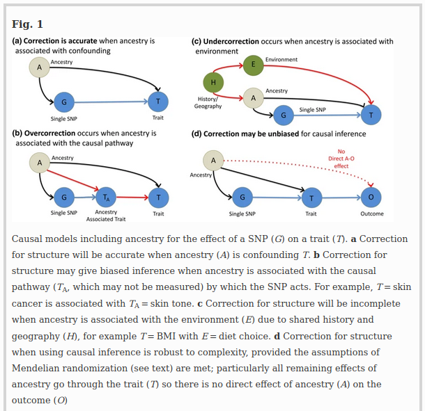
A central goal of genetic association studies is to estimate the “true” causal effect of a SNP (G) on a trait (T). The “true” effect is defined as the effect of G on T when all other traits that are not in the pathway between G and T (i.e., confounders) are accounted for (Fig. 1). Correction of GWAS for ancestry (A) is designed to remove non–causal associations when observable ancestry (CA, which might be PCs) not in the causal pathway (Fig. 1a). However, it also removes causal associations when ancestry is associated with traits in the pathway (Fig. 1b); a phenomenon often called vertical pleiotropy. Corrected estimates of the G–T associations exclude the G–A–T association. However, they also exclude the G–TA–T association and hence may under-estimate the effect size. For example, if G increases the risk of skin cancer by changing skin tone, its effect size will be underestimated if skin tone is predicted by ancestry. In general, because modern populations are mixtures of ancient populations, many SNPs with a biological effect (including ADH1B and Lactase) may associate with ancestry PCs due to having been common in only one ancestral population.
This is the same thing we have been saying for a while, citing the example of induced selection in the Russian Fox Experiment (see post: FAQ for Dunkel et al 2019 Ashkenazim polygenic score for intelligence).
Simulating phenotypes with population stratification
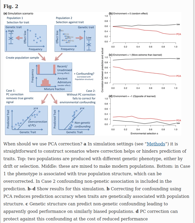
For genome-wide questions including heritability analyses and prediction, it is easy to construct scenarios in which either correction or non-correction for structure can be misleading. Figure 2 describes two simulation scenarios: case 1 in which true genetic signal for a trait is associated with population structure (e.g., height), and case 2 in which population structure associates non-causally with the trait through the environment. PC correction is conservative when phenotypes are truly associated with ancestry (Fig. 2b). When ancestry is predictive of the environment (Fig. 2c) it can even increase genetic associations through non-causal pathways. However, when genes have moved into new environments, PC correction reduces bias (Fig. 2d).
Oddly:
It is unclear how many of these GWAS hits are in fact hits for ancestry and hidden population structure or migration. The problem exists in many other phenotypes (Martin et al. 2017): for example “height is predicted to decrease with genetic distance from Europeans” which is not empirically observed. Interpretation of these results is left to the discussion.
Pretty sure this is empirically observed. Europeans are tall, some other groups are also tall, but overall, they are shorter. Someone can plot the results from national Fst and height data.
Variation between populations can be exploited as part of the statistical methodology, to further learn about the genetic structure of a phenotype. Within a population, admixture mapping was an early tool (Winkler et al. 2010) to exploit variation in ancestry, though there are relatively few recent novel discoveries using this method, one being Adhikari et al. (2016). Across populations, standard GWAS methodology has been successfully applied and extended in “trans-ethnic” approaches (Li and Keating 2014) which start by treating ancestry as a fixed or random effect in regression. More sophisticated approaches such as MANTRA (Morris 2011) and MR-MEGA (Mägi et al. 2017) model heterogeneity in ancestry-specific effects, allowing the agreement between different populations to be measured. Popcorn (Brown et al. 2016) allows this to be done using only GWAS summary statistics. The consistent story across all phenotypes studied in these papers—rheumatoid arthritis, type 2 diabetes, gene expression, and kidney function—is that that both environment and ancestry play an important a role in explaining differences in populations. The total contribution of both is usually on the same order of magnitude. Although not conclusive in human studies, gene–environment interactions have also been explicitly measured and can contribute substantially, e.g., adding 11% to accuracy in a plant study (Desta and Ortiz 2014).
And now for the most important part:
The educational attainment results highlighted by structure within the ALSPAC study reveal important complexity. The effect sizes in trio studies (Okbay et al. 2016) are theoretically not confounded by population structure, and are consistently 30–40% smaller than the inferred effects for the larger, unrelated sample. Our results show that population structure alone can predict educational outcome better than was previously thought. It is still unclear how this predictive power arises—this study implicates migration whilst other explanations include assortative mating and dynastic effects (Kong et al. 2018; Young et al. 2018), as well as sampling biases, though these are not mutually exclusive. We have discussed reasons to adjust GWAS results—or not—using higher quality ancestry estimates for the consortium datasets. There are two opposing hypotheses, which are both consistent with the available data:
- (a) Educational attainment is associated with ancestry because of causal pathways that should be included in our definition of the phenotype. For example, historical biased migration could create “brain drain”, or selection on ancestral populations leading to a difference in ability (Clark and Cummins 2018). Alternatively, phenotypic differences between populations might exert influences over life-choices.
- (b) Educational attainment is associated with ancestry because of non-causal phenotypic pathways. Examples include access to education, cultural norms, the relationship between education and GDP (Nelson and Phelps 1966), and discrimination within the educational system (Light and Strayer 2002; Song 2010).
It is likely that a combination of the above is true. Non-causal pathways are certainly plausible (Fig. 5): average education levels and GDP per capita are correlated within countries and between countries in Europe (Mankiw et al. 1992). GDP is in turn correlated in Northern Europe and the UK with high Germanic and Scandinavian ancestry, such as England, Germany, Denmark, Netherlands, Belgium and Luxembourg.
And there we have it, ancestry is likely part of the explanation for varying educational attainment, and by implication, intelligence, GDP per capita and everything else between parts of Europe with high Germanic ancestry, and other parts. Naturally, there are 0.000000 citations of any of the people who have been arguing the same things for decades based on other evidence (general principle: Thou shall not cite Richard Lynn). For instance, take a look at the paper in this post.