Over at SlateStarCodex AstralCodexTen commenter Himaldr asked me:
>”because strength of the correlation has a linear relationship with the expected return of using it for selection (hiring) purposes.”<
Can you expand upon this a bit, if you get a chance? It seems to me that ought not be the case — but perhaps I misunderstand “expected return” in this context (in terms of winnowing candidates? in terms of quality of work?), or else something else in my mental model is dumb and wrong.
(e.g.: taking Brandon’s example, but pretending “statsophrenia” is actually very desirable, is knowing a candidate’s genetic risk factor only twice as valuable as knowing their environmental risk…?)
I wrote a brief reply there, but it is worth hammering home the point for future reference. The industrial psychologist duo John Hunter and Frank Schmidt were (some of) the first to figure out how to calculate the dollar value of selection in hiring. Hunter developed an equation for this, which is presented in his 1984 article (with his wife) Validity and Utility of Alternative Predictors of Job Performance (PDF). In the article they write:
Economic Benefits of Various Selection Strategies
Differences in validity among predictors only become meaningful when they are translated into concrete terms. The practical result of comparing the validities of predictors is a number of possible selection strategies. Then the benefit to be gained from each strategy may be calculated. This section presents an analysis of the dollar value of the work-force productivity that results from various selection strategies.
…
A number of methods have been devised to quantify the value of valid selection (reviewed in Hunter, 198la). One method is to express increased productivity in dollar terms. The basic equations for doing this were first derived more than 30 years ago (Brogden, 1949; Cronbach & Gleser, 1965), but the knowledge necessary for general application of these equations was not developed until recently (Hunter, 1981a; Hunter & Schmidt, 1982a, 1982b; Schmidt, Hunter, McKenzie, & Muldrow, 1979). The principal equation compares the dollar production of those hired by a particular selection strategy with the dollar production of the same number of workers hired randomly. This number is called the (marginal) utility of the selection procedure. Alternative predictors can be compared by computing the difference in utility of the two predictors. For example, if selection using ability would mean an increased production of $ 15.61 billion and selection using biodata would mean an increased production of $10.50 billion, then the opportunity cost of substituting biodata for ability in selection would be $5.11 billion.
…
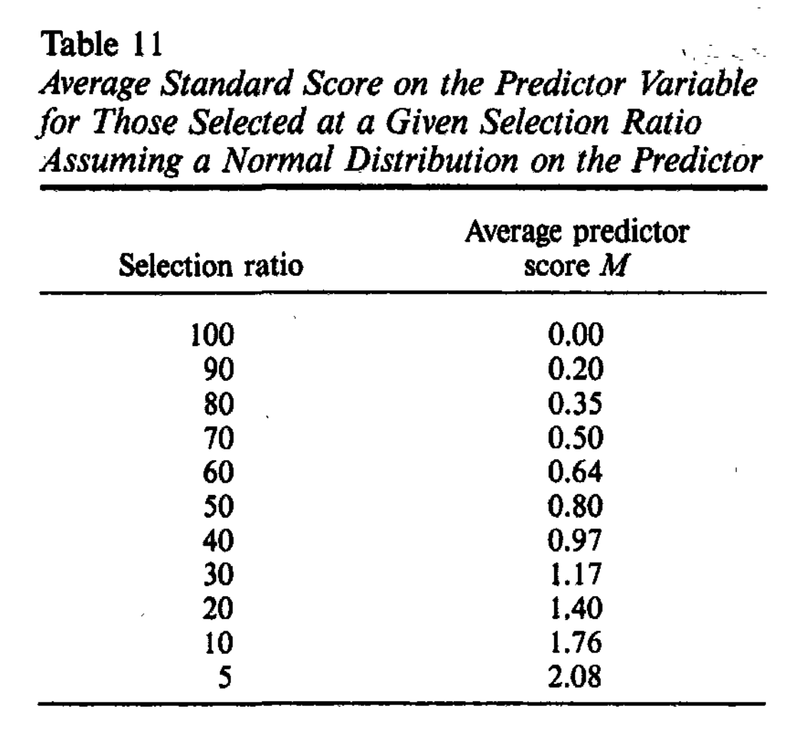
This completes the list of administrative factors that enter the utility formula: N = the number of persons hired, T = the average tenure of those hired, SDy = the standard deviation of performance in dollar terms, and M = the expression of the selection ratio as the average predictor score in standard score form. One psychological measurement factor enters the utility equation: the validity of the predictor, rxy, which is the correlation between the predictor scores and job performance, for the applicant or candidate population. If this validity is to be estimated by the correlation from a criterion-related validation study, then the observed correlation must be corrected for error of measurement in job performance and corrected also for restriction in range. Validity estimates from validity generalization studies incorporate these corrections. The formula for total utility then computes the gain in productivity due to selection for one year of hiring:
U = N * T * r_xy * SDy * x_mean
To showcase this, we can run a simulation. Suppose you have a company and you want to hire 10 people. You post a job ad somewhere, and you get 100 applicants who seem to resemble the generation population, so you get to hire the 10% best people. But how exactly? You need some kind of hiring procedure. You could do interviews, but do you really want to interview 100 different people? That takes a long time, or costs a lot of money if you outsource it (i.e., pay someone to do this). So instead, you come up with some kind of objectively scored test that you can give to everybody in a single setting (a group test). It need not be a strict intelligence (IQ) test, it can involve knowledge of the business field you are in (job knowledge tests). Based on prior research, you figure this test has a validity of .40, that is, the test score correlates .40 with job performance.
After getting the 100 applicants to take your test, you find this result:
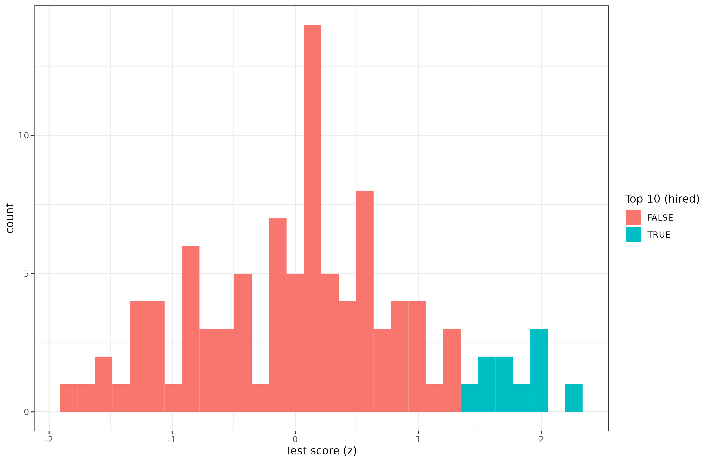
The average test score of those you hired was 1.79 z, or the 96% centile. How much higher were they in job performance when you later did the reviews? The mathematical expectation is just 0.40 * 1.79 = 0.72, so they should be above average workers. But almost every decision in life has some chance element to it. Maybe you got lucky or unlucky. The actual average job performance score was 0.77, however, so you were slightly on the lucky side.
If we run this thought experiment 100 times, we can see the average or expected benefit of using this hiring procedure:
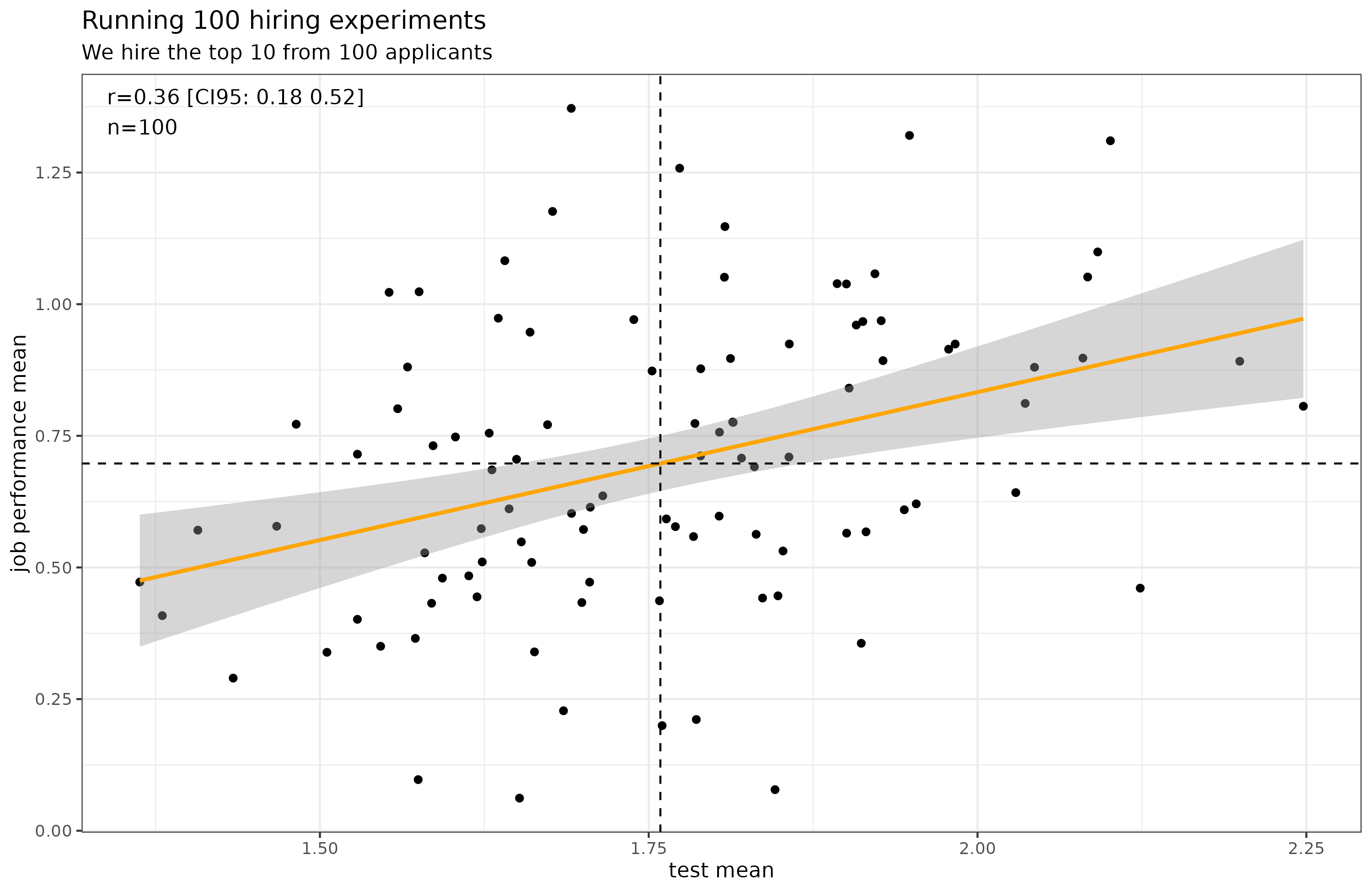
Thus, on average, you would expect to find that the hired people have a mean test score of 1.76, and a mean job performance of 0.70. In other words, using this approach, you would hire people who were 0.70 standard deviations better than if you had been hiring people at random or using an invalid (r = 0) procedure. This value of 1.76 is fortunate because that’s the same value we can find in the paper under the selection ratio of 10:
How much is this in dollars, though? You need to know how job performance translates to dollar value for your job. The Hunters write:
The standard deviation of job performance in dollars, SDy, is a difficult figure to estimate. Most accounting procedures consider only total production figures, and totals reflect only mean values; they give no information on individual differences in output. Hunter and Schmidt (1982a) solved this problem by their discovery of an empirical relation between SDy and annual wage; SDy is usually at least 40% of annual wage. This empirical baseline has subsequently been explained (Schmidt & Hunter, 1983) in terms of the relation of the value of output to pay, which is typically almost 2 to 1 (because of overhead). Thus, a standard deviation of performance of 40% of wages derives from a standard deviation of 20% of output. This figure can be tested against any study in the literature that reports the mean and standard deviation of performance on a ratio scale. Schmidt and Hunter (1983) recently compiled the results of several dozen such studies, and the 20% figure came out almost on target.
So let’s say your workers get paid 50k USD a year. In that case, we may surmise the standard deviation of job performance in dollar values is 50k * 0.4 = 20k. Using this procedure, then, will on average yield a value of 20k * 10, or 200k USD/year, as you hired 10 people.
Does this standard deviation value hold up, though? This result is from an 1983 meta-analysis based on even older studies. I’ve heard about the 10x programmer, is this true? Well, Hunter, Schmidt and Judiesch did a 1990 meta-analysis looking into job complexity as a moderating factor (Individual differences in output as a function of job complexity), and they found:
The hypothesis was tested that the standard deviation of employee output as a percentage of mean output (SDp) increases as a function of the complexity level of the job. The data examined were adjusted for the inflationary effects of measurement error and the deflationary effects of range restriction on observed SDp figures, refinements absent from previous studies. Results indicate that SDp increases as the information-processing demands (complexity) of the job increase; the observed progression was approximately 19%, 32%, and 48%, from low to medium to high complexity non-sales jobs, respectively. SDp values for sales jobs are considerably larger. These findings have important implications for the output increases that can be produced through improved selection. They may also contribute to the development of a theory of work performance. In addition, there may be implications in labor economics.
So the initial results hold up fairly well. But for sales occupations and high end complexity jobs (say, computer science startups), you will probably want to use a larger SD in the equation. In fact, there is a researcher called Herman Arguinis who argues that many job performance distributions follow a power law (“star performer”), and if so (and not everybody agrees), the utility gains from selection become much larger and more difficult to calculate directly (but can be done from simulations).
Going back to my original point with the comment. The point is that correlations are the right metric for measuring the importance of something, not correlations squared or any other variance metric. These are deceptive. Schmidt and Hunter explain it thus in their meta-analysis book:
Variance-based interpretations have led to the same sort of errors in personnel selection. There it was said that validity coefficients of, for example, .40 were not of much value because only 16% of the variance of job performance was accounted for. A validity coefficient of .40, however, means that, for every 1 SD increase in mean score on the selection procedure, we can expect a 0.40 SD increase in job performance—a substantial increase with considerable economic value. In fact, a validity coefficient of .40 has 40% of the practical value to an employer of a validity coefficient of 1.00—perfect validity (Schmidt & Hunter, 1998; Schmidt, Hunter, McKenzie, & Muldrow, 1979).
As I have explained before, the same is true when it comes to polygenic embryo selection, which is essentially a hiring task for the job of being your child. 🧒🏻