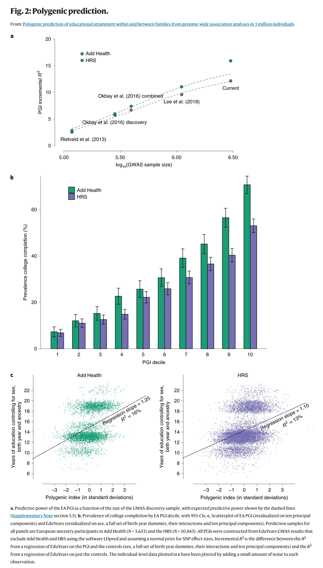
- Okbay, A., Wu, Y., Wang, N., Jayashankar, H., Bennett, M., Nehzati, S. M., … & Young, A. I. (2022). Polygenic prediction of educational attainment within and between families from genome-wide association analyses in 3 million individuals. Nature Genetics, 1-13.
We conduct a genome-wide association study (GWAS) of educational attainment (EA) in a sample of ~3 million individuals and identify 3,952 approximately uncorrelated genome-wide-significant single-nucleotide polymorphisms (SNPs). A genome-wide polygenic predictor, or polygenic index (PGI), explains 12–16% of EA variance and contributes to risk prediction for ten diseases. Direct effects (i.e., controlling for parental PGIs) explain roughly half the PGI’s magnitude of association with EA and other phenotypes. The correlation between mate-pair PGIs is far too large to be consistent with phenotypic assortment alone, implying additional assortment on PGI-associated factors. In an additional GWAS of dominance deviations from the additive model, we identify no genome-wide-significant SNPs, and a separate X-chromosome additive GWAS identifies 57.
So it is finally out. The new GWAS, EA4, the fourth iteration for educational attainment. It now has some 3 million Europeans, and which improved the prediction accuracy a bit. The main paper is relatively short, 31 pages, the supplement is a whopping 104 pages, and there’s a file with 30 supplementary tables. So let’s dive in!
The sample size is now about 3 times larger, but actually all of the increase comes from 23andme collecting/sharing more data. Thus, consumer genomics is actually driving research into genetics of intelligence. With the improved sample size, the authors basically used the same method as before. GWASs (genome-wide association study) are really very rudimentary models. The sensible approach of building a predictive model is to pick a good machine learning algorithm (actually multiple), feed all the genetic variants data into it, and tell it to predict education/intelligence/whatever, with results verified by k-fold cross-validation. This is NOT what is done. Instead, researchers fit a linear model with 1 focal genetic predictor at a time in each dataset/cohort, of which there are about 70. They usually include some controls, which are typically age, sex, and principal components meant to control for any residual ‘population stratification’. Since the arrays used to measure genetic variants are different between datasets, and thus measure different variants, researchers fill in unmeasured variants based on the ones they measured (imputation, that’s what impute.me does when you upload your 23andme to it). This results in about 10 million variants measured or estimated on the non-sex chromosomes (autosomes). After the filling in is done, the regressions are run. This then results in about 70 sets of 10 million regression results with one variant at a time. Then, for each variant, they meta-analyze the results across the datasets, thus resulting in about 10 million regression model meta-analyses. That’s the GWAS output, those called summary statistics that you can download for free cannot download due to censorship. Actually, since 23andme is obnoxious, the EA4 group only published about 10,000 of the most important and most independent genetic variant results. These are the ones other researchers get to use. They can do their own application at 23andme to get the full list (naturally, this excludes anyone doing research disliked by the mainstream). The Table 1 in the EA4 paper shows the progress in sample size over the years.

Each genetic variant is assigned a p value based on the meta-analysis, which measures how unlikely the association is if we assume the variant is not actually associated with education. You can think of it as a certainty of signal value, though it does not measure the strength of the association, just whether we can be sure there is some association. We can plot these p values to get the typical Manhattan plot:

The y axis shows a recoding of the p value so that it is more sensible than looking at values like 0.00000000000000003. Simply, it’s the -log10(p), which just counts how many decimal zeros are in the p value. So for the above number, this value is 16.5. Why is this needed? Why not use the trusted 0.05 standard? Well, because when you test 10 million variants, you have 10 million chances to get a low value by coincidence, and the easy fix for this is to decrease the threshold to account for this. This is how they derived the ‘genome-wide significance’ threshold which is the dotted line you see above (among the green dots). All the dots above that line are variants showing associations greater than chance would predict, even taking into account that we tested so many million variants. As you can see, there are thousands of such dots. I was unable to figure out how many there actually are, which is to say: which proportion of tested variants show a signal? The greater the value, the more spread out the genetic signal is. Human intelligence is the most complex on the earth, and took millions of years to fine-tune, so it is not so surprising it depends on the combined variation in 10,000+ genetic variants.
The authors then did some filtering, called clumping. What this means is that they go over the genome in small regions, and within each region, they pick the variant showing the best association based on multiple criteria, but mainly its p value being the lowest. There are more advanced methods for this, which is the area of research called fine mapping. In this approach, one attempts to figure out which variants are causal based on things like the nature of the variant, known pathways, expected effects on the proteins/promoters, and so on. The end result of the simple and advanced methods is that one ends up with a set of relatively unrelated, plausible genetic variants, called the lead SNPs in the paper (they are probably not all SNPs, some are usually indels, which are short insertions or deletions; SNPs are single variant changes, e.g. a T or an A at some location). This number of lead variants is the one that has now reached almost 4,000 using the ‘lenient’ p value threshold, and about 3,300 with a stricter one.
Next up, the authors repeat this ordeal but for the X chromosome. This requires some recoding so that men’s 1 copy is comparable to women’s 2 copies. After this, they find another 57 lead variants on the X chromosome. They also did this for each sex independently to see if the X chromosome results are near-identical across sexes, which they were (genetic correlation .94, se = .03). This just tells us what we already knew, i.e., that the X chromosome is not particularly important for intelligence.
The more interesting thing is that they looked for non-linear effects of genetic variants. Mathematically, this is merely asking whether having 2 copies of the minor allele (the less common version of some genetic variant) is twice as effective as having 1 copy. So for height, if having 1 copy of some allele makes you 1 cm taller, then having 2 copies should make you 2 cm taller, both in compared to those who have 0 copies. They find that… this never occurs across the about 6 million variants they tested! They show that they had sufficient statistical precision to find such effects if they had existed and had sizes that are worth caring about. This is an unexpected finding! Everybody knows that inbreeding is bad, and inbreeding being bad results from such non-linear effects. In disease genetics, these are called dominant and recessive effects. Most severe genetic disorders are recessive, meaning that you need to have 2 copies of a bad allele to get the disorder, while 1 copy does nothing by itself (i.e., a non-linear effect). Somehow this is not found for any of those 6 million variants. I can think of a few interpretations: 1) we don’t have as much statistical precision as we think we have, 2) inbreeding isn’t as bad as we think it is, 3) the non-linear effects are there but not for these kinds of genetic variants. I don’t think (1) is plausible given the huge sample, and the authors do formal power calculations to back this up. For (2), we have verified that inbreeding is bad by actual breeding experiments with animals, and there’s also that thing called the Habsburg family trial. So that leaves us with (3), which is also what the authors go for. The included variants are mostly SNPs, and not larger deletions, or inversions etc., which presumably are more commonly the cause of major diseases. These are also quite rare, so they can’t be imputed accurately with the array data we have. This is kind of a genetics of the gaps argument, so it leaves a bad epistemic taste in the brain-mouth, but what else do we conclude here?
Finally, we get to the more interesting part: polygenic scores. They call them polygenic indexes, which is the current thing (euphemism) in GWASs.

For validation, they have 2 datasets they didn’t use for training the model. The first part of the plot shows the increase in the validity of these scores across the iterations of education GWASs, with the x axis showing the log10 sample size (number of zeros in the sample size). The improvement looks relatively log-linear (linear when you log transform x), which is BAD.

Suppose we take the most optimistic results based on the Add Health dataset. We get 17% incremental R2 in EA4. We can then ask: how many million people do we need to predict 50% of the variance? We can eyeball the data from their plot, and make a simple linear model. This is of course really a more logistic function, but a linear fit has an R2 of 95%, so let’s roll with it as a starting point. The answer is that we need log10 n of 10, that is, 10,000,000,000 people. That’s 10 billion, which is… every human on the planet! Now, humans replenish, so we can measure all humans, then wait a decade or three, then we can measure the new ones too and improve our sample size over the decades. But really, we need something far far better.
The current hopes are 1) improved modeling approaches, 2) whole genome sequencing. The latter will give us a lot more variants, including new types that we currently ignore. There is evidence that such currently unused variants can have large effects, so we can expect a reasonable boost just from their inclusion. Second, we will be measuring all variants directly, instead of imputing them which has an error associated with it. This is especially important for the more rare variants, which are thought to have potentially large effects. What about improved modeling approaches? Why the hell do geneticists use such a dumb approach as the one I outlined above?? It’s because they aren’t allowed to share the datasets directly. That’s why every group that contributes data does so independently. This terrible approach is why one has to rely on hack-methods that approximate the elastic net using summary statistics alone (SBayesR, LDpred etc.). We can only hope that future datasets will be more shareable, and larger so that single datasets will allow for proper machine learning approaches. There is hope toward this end because the UK Biobank (about 500k persons) is already such a single dataset, and it is currently being sequenced, so whole genome data will be forthcoming. Furthermore, studies already show that using proper learning algorithms on this dataset can improve the validity quite a lot. The second hope is the American Million Veterans Program.
Anyway, to return the EA4 results. The authors then show that aside from predicting education with the new polygenic scores, one can also use them to predict other traits. This is because of the fact that education, and it’s causes (intelligence chiefly) also predict or cause many other traits, so one can rely on the indirect validity. Some phenotypes also share genetic variants, so therefore a prediction for one phenotypes is a prediction in part for another phenotypes (pleiotropy).

This general approach of using many polygenic scores to predict phenotypes has been shown to be correct in various studies.
More on the applied side, they report the validity among sibling pairs. Validity among siblings is very important because it cannot be due to family-level confounding factors, which include population stratification, and just about everything else sociologists have been claiming for the last 10 decades. The authors take their education predictive model and compare it with other genetic models for height, BMI, and intelligence. They find that education model loses the most accuracy when using siblings.

How is this interpreted? I can think of 2 main explanations: 1) the EA genetic prediction score is really indexing quite substantively some family-level factors we didn’t properly control for, and so it is overestimating genetic effects. This is expected because educational attainment has the largest shared environment component of these traits according to twin studies, about 30%. This also includes complicated stuff like genetic nurture, which is all the rage these years. 2) We didn’t adjust for assortative mating. Assortative mating makes siblings more genetically similar for the assorted phenotype than expected (more than .50 correlated). I am not exactly sure how this would affect the ratio of the between/within family slope, but maybe it would. As a matter of fact, the same assortative mating bias inflates the shared environment estimates from twin studies, so it may be more like 10-20% for education even.
Speaking of assortative mating, the authors then show this is a lot stronger for the polygenic score for education than expected based on the observed phenotypes. What this means is that people aren’t assorting so much on observed educational attainment, they are assorting on the causes of educational attainment, the human capital traits directly. This is really what Gregory Clark has been saying all along. His work finds that assortative mating is really strong, even back when women didn’t work much outside the home, or got much education. Plausibly then, couples were then assorted on these various psychological traits that make up human capital. This is the same as the latent S factor in my formulation.

In fact, there is another recent paper using a good SEM approach, and which finds much the same:
- Torvik, F. A., Eilertsen, E. M., Hannigan, L. J., Cheesman, R., Howe, L. J., Magnus, P., … & Ystrom, E. (2022). Modeling assortative mating and genetic similarities between partners, siblings, and in-laws. Nature communications, 13(1), 1-10.
Assortative mating on heritable traits can have implications for the genetic resemblance between siblings and in-laws in succeeding generations. We studied polygenic scores and phenotypic data from pairs of partners (n = 26,681), siblings (n = 2,170), siblings-in-law (n = 3,905), and co-siblings-in-law (n = 1,763) in the Norwegian Mother, Father and Child Cohort Study. Using structural equation models, we estimated associations between measurement error-free latent genetic and phenotypic variables. We found evidence of genetic similarity between partners for educational attainment (rg = 0.37), height (rg = 0.13), and depression (rg = 0.08). Common genetic variants associated with educational attainment correlated between siblings above 0.50 (rg = 0.68) and between siblings-in-law (rg = 0.25) and co-siblings-in-law (rg = 0.09). Indirect assortment on secondary traits accounted for partner similarity in education and depression, but not in height. Comparisons between the genetic similarities of partners and siblings indicated that genetic variances were in intergenerational equilibrium. This study shows genetic similarities between extended family members and that assortative mating has taken place for several generations.
Their model looks like this:

Their results:

Clark’s most recent paper on this is this one:
- Clark, G., & Cummins, N. (2022). Assortative Mating and the Industrial Revolution: England, 1754-2021.
Using a new database of 1.7 million marriage records for England 1837-2021 we estimate assortment by occupational status in marriage, and the intergenerational correlation of occupational status. We find the underlying correlations of status groom-bride, and father-son, are remarkably high: 0.8 and 0.9 respectively. These correlations are unchanged 1837-2021. There is evidence this strong matching extends back to at least 1754. Even before formal education and occupations for women, grooms and brides matched tightly on educational and occupational abilities. We show further that women contributed as much as men to important child outcomes. This implies strong marital sorting substantially increased the variance of social abilities in England. Pre-industrial marital systems typically involved much less marital sorting. Thus the development of assortative marriage may play a role in the location and timing of the Industrial Revolution, through its effect on the supply of those with upper-tail abilities.
Thus, Clark found that latent assortative mating is about .80 for occupational status, whereas Torvik et al estimated this value to be about 0.68 for education. Since education is only one component of occupational status (or the more general S), these values are pretty compatible.
Conclusions
EA4 represents a solid, but incremental step forward. We really need get serious about whole genome sequencing, larger samples, more use of family members to avoid unobserved familial confounding, proper data sharing resulting in machine learning, and the use of multi-ethnic/mixed ancestry samples. The latter is of course where the bogeyman hides is plainly standing, since there are many inconvenient findings in this area. We have already showed that genetic ancestry explains most intelligence differences between African Americans and European Americans (papers ½, 1, 2, 3, 4), and that these are partially mediated by the current polygenic scores. As these genetic predictive models continue to improve, the mediation will be stronger. Davide Piffer and I are working on the next iteration of the global comparisons, this time with a much expanded set of populations. The first part will be a study of the Italian north-south gaps. We find that polygenic scores reveal these as well, which is not very surprising given that all the indirect evidence was in that direction already. Stay tuned and subscribe for more!